Bench Degree·SOLAR POWERchapter

Chapter 7: The I-V Curve, and the Only Point That Matters
A panel produces exactly zero watts at both ends of its own range: nothing when open circuit, nothing when short circuit. Everything useful happens at one bend in the middle, and finding that bend is a whole product category.
Two numbers are printed on every solar panel and quoted in every advertisement: open-circuit voltage and short-circuit current. Take the 100 W panel from Chapter 1, which reads 22.0 V open and 6.10 A shorted.
Multiply them. 22.0 x 6.10 = 134 W.
The panel is labelled 100 W.
Now measure the power at each of those two conditions instead of multiplying them together. Open circuit: 22.0 V, and no current, because nothing is connected. Power = 0 W. Short circuit: 6.10 A, and no voltage, because the terminals are joined. Power = 0 W.
The panel delivers nothing at either of the two numbers on its label. Both of the figures everybody quotes are points of zero output. What you need is a specific place between them, and the only way to find it is to put a load on the panel and vary it.
So do that.
Wire a rheostat across the panel, put a voltmeter across the panel and an ammeter in series with it, and walk the resistance from a dead short up to open circuit, writing down voltage and current at each step. Multiply each pair. Here is what the Chapter 1 panel gives on a clear day at noon:
| Load (Ω) | Volts | Amps | Watts |
|---|---|---|---|
| short | 0 | 6.10 | 0 |
| 1.0 | 6.05 | 6.05 | 36.6 |
| 2.0 | 12.0 | 6.00 | 72.0 |
| 2.5 | 14.7 | 5.88 | 86.4 |
| 3.0 | 17.2 | 5.73 | 98.6 |
| 3.24 | 18.0 | 5.56 | 100.1 |
| 3.5 | 18.6 | 5.31 | 98.8 |
| 4.0 | 19.4 | 4.85 | 94.1 |
| 6.0 | 20.6 | 3.43 | 70.7 |
| 10 | 21.3 | 2.13 | 45.4 |
| 20 | 21.7 | 1.09 | 23.6 |
| 50 | 21.9 | 0.44 | 9.6 |
| open | 22.0 | 0 | 0 |
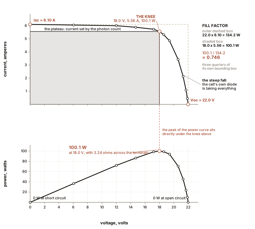
There it is. Power climbs from zero, peaks at 100.1 W with 3.24 Ω across the terminals, and falls back to zero. The peak is sharp on one side and gentle on the other, and it is nowhere near the middle of the voltage range.
ON THE BENCH: Trace your own I-V curve by hand
Parts: a panel of 10 to 100 W; a wirewound rheostat, 50 Ω and at least 50 W rating, about $20; two or three fixed power resistors of 1, 2 and 3 Ω, about $3 each, for the low-resistance end where the rheostat is coarse; two multimeters; graph paper. Cost: about $30 if you own one meter and borrow another. Time: two hours, and pick a cloudless day so the sunlight does not change under you. Hazards: the rheostat will get hot enough to burn you at the low-resistance end, because it is dissipating the panel’s entire output. Mount it on something that will not scorch and do not touch the wiper. Method: voltmeter across the panel, ammeter in series with the load. Start with the rheostat at maximum and work down, then switch to the fixed resistors for the last few points, then short the ammeter straight across the panel for the final one. Work fast and check the open-circuit voltage every few minutes; if it has drifted, the sun or the panel temperature has changed and your curve is smeared across two conditions. Then plot two graphs on one sheet: current against voltage, and power against voltage. The first is the I-V curve. The second has a clear peak, and its location is the answer to this chapter. What you should see: a curve that is nearly flat at the short-circuit current out to perhaps 70 percent of the open-circuit voltage, then a knee, then a steep fall to zero. Peak power between 70 and 80 percent of open-circuit voltage. If your peak is much lower than the nameplate: it almost certainly is, and the panel is not faulty. It is hot, and Chapter 9 is about exactly how much that costs. Measure the back of the panel with an infrared thermometer while you work and write the temperature next to every reading.
Section 1: Reading the Curve
Five numbers describe the whole thing, and every datasheet in the industry lists all five.
Isc, short-circuit current. 6.10 A here. Set purely by photon count, as Chapter 4 showed, so it tracks sunshine almost perfectly linearly. It is the most honest number on a datasheet.
Voc, open-circuit voltage. 22.0 V. Set by the material and the number of cells in series, as Chapter 6 showed, and barely moved by how bright the light is. It moves a great deal with temperature.
Vmp, voltage at maximum power. 18.0 V. About 82 percent of Voc on this panel; typically 75 to 85 percent.
Imp, current at maximum power. 5.56 A. About 91 percent of Isc.
Pmax. 100.1 W, being Vmp times Imp, and it is the number on the label.
Then one derived figure that tells you more about the panel’s quality than any of the others.
Fill factor is how close the curve comes to the rectangle that Voc and Isc would enclose if the panel were perfect:
FF = Pmax / (Voc x Isc) = 100.1 / 134.2 = 0.746Seventy-five percent. The curve fills three quarters of its bounding box. A good modern module manages 0.79 to 0.82; a cheap one 0.70 to 0.75; anything below 0.65 has something wrong with it, usually series resistance in the contacts or a shunt path across a cell.
IN PLAIN ENGLISH: A solar panel is not like a battery, which holds its voltage and gives you whatever current you draw. It is more like a person carrying a stack of plates: ask for a reasonable number and you get them, ask for too many and they drop the lot. The panel will supply up to about six amps at almost any voltage below eighteen. Ask for more current than that and the voltage collapses instead. The best deal is right at the edge, and the edge moves as the light and the temperature change.
Section 2: Where the Knee Comes From
The knee is not a manufacturing artefact. It is the diode of Chapter 6 turning on.
Recall the model: I = IL - I0 x (exp(V / (n x Vt)) - 1).
The first term is the photocurrent, constant. The second is the cell’s
own diode, forward biased by whatever voltage the cell finds itself
at.
At low voltage that exponential is negligible, so the current out is simply the photocurrent, and the curve is flat. Every generated pair is leaving through the wire.
As voltage rises, the diode begins to conduct, and the current it passes is current that never reaches your load. It goes round inside the cell instead, an electron falling back into a hole rather than travelling through the external circuit.
The knee is the voltage at which the cell’s own diode starts stealing meaningfully from your load, and beyond it the theft grows exponentially. At open circuit the diode is taking all of it, which is exactly why the output is zero there.
So a solar cell in operation is a competition between a photon-driven current going out and a voltage-driven recombination current going round in circles, and the maximum power point is the best terms you can get in that competition.
Section 3: What Direct-to-Battery Costs You
Now the practical consequence, and it is expensive.
Connect that panel directly to a 12 V lead-acid battery, which is the simplest possible solar charging arrangement and how millions of caravans, boats and gate openers are wired.
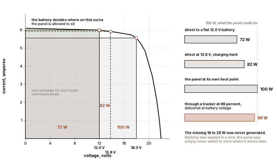
The battery sets the voltage. It does not care what the panel would prefer. A battery at mid charge sits near 12.4 V; charging hard it might be pulled to 13.8 V; deeply discharged, 12.0 V.
Read those voltages off the table.
At 13.8 V the panel supplies about 5.92 A, so
13.8 x 5.92 = 82 W. At 12.0 V the panel supplies 6.00 A, so
12.0 x 6.00 = 72 W.
The panel was capable of 100 W. It is delivering 72 to 82 W, and the missing 18 to 28 W was never generated at all. It is not lost in a wire or burned in a resistor. The panel simply was not asked to operate where it works best, so it did not.
A maximum power point tracker fixes this by refusing to let the battery set the panel’s voltage. It presents the panel with whatever load makes it sit at 18.0 V, takes the full 100 W, and then converts that 100 W down to whatever voltage the battery needs, using a switching converter that is typically 95 to 97 percent efficient.
100.1 W x 0.96 = 96 W delivered to the battery.
So the honest comparison:
| Battery state | Direct connection | With MPPT | Gain |
|---|---|---|---|
| Deeply discharged, 12.0 V | 72 W | 96 W | 33 percent |
| Mid charge, 12.4 V | 74 W | 96 W | 30 percent |
| Charging hard, 13.8 V | 82 W | 96 W | 17 percent |
The “thirty percent” that MPPT controllers are marketed on is the best case, not the typical one. It is true when the battery is flat and the panel is cold. When the battery is nearly full and the panel is hot, the gain can fall to ten percent or less, because a hot panel’s Vmp drops toward the battery voltage and the mismatch shrinks.
That last sentence contains something worth noticing. The value of MPPT depends on temperature, and it is largest exactly when a panel performs best, on cold bright days. In a cold climate the gain is real and consistent. In a hot one it is smaller than the box promises.
ON THE BENCH: MPPT against direct, same panel, same day
Parts: a panel of 50 to 100 W; a 12 V lead-acid battery, partly discharged; a PWM charge controller, about $15; an MPPT charge controller, about $60; two clamp meters or two multimeters; an infrared thermometer, about $20. Cost: about $100, and the controllers keep their value. Time: an afternoon. Hazards: lead-acid batteries vent hydrogen when charging and will deliver hundreds of amps into a dropped spanner. Work outdoors, fuse the battery lead, remove rings and watches. Method: run the panel through the PWM controller into the battery for fifteen minutes, measuring panel voltage, panel current, battery voltage and battery current. Swap to the MPPT controller and repeat immediately, in the same sun, at the same battery state of charge. Record the panel’s back-surface temperature both times. What you should see: with PWM, panel voltage pulled down to within a volt of the battery. With MPPT, panel voltage sitting near its Vmp, and battery current higher by somewhere between 10 and 35 percent. The measurement that makes the point: compute panel watts (panel volts times panel amps) in both cases. With PWM, the panel itself is producing less. That is the entire lesson: nothing was wasted downstream, the generation never happened. If the MPPT controller shows no advantage: many cheap controllers sold as MPPT are PWM inside. Check whether panel voltage actually differs from battery voltage while it is running. If it does not, you have bought a label.
Section 4: How a Tracker Actually Finds the Knee
The knee moves. It moves with irradiance, with temperature, and with shading, so a tracker cannot be set once at the factory. It has to search, continuously, forever.
The dominant method is called perturb and observe, and it is disarmingly simple.
Nudge the operating voltage up slightly. Measure the power. If power went up, nudge the same way again. If power went down, nudge the other way. Repeat a few times per second, forever.
That is it. It converges on the peak from either side, it needs no model of the panel, and it works on any panel ever made. Its one flaw is that at the exact peak it cannot tell which way to go, so it oscillates gently around the maximum, giving up a fraction of a percent in exchange for never needing to be told anything about the hardware.
Incremental conductance is the refinement: instead of comparing power before and after, it computes the slope of the power curve and steps proportionally to how far from the peak it appears to be. Faster on rapidly changing days, more sensitive to noisy measurements.
Both share one serious weakness, and Chapter 9 will make a great deal of it. A partially shaded string has more than one peak on its power curve, and a hill-climbing algorithm finds the nearest one, which may not be the highest. A tracker sitting confidently on a local maximum while a much better one exists 80 V away is a real and common failure mode, and it is why good inverters periodically sweep the entire voltage range rather than trusting the hill they are on.
Section 5: Why This Chapter Sets Up the Rest of the Book
Three things carry forward.
Nameplate power is a point, not a property. It is the peak of one curve measured under one set of laboratory conditions. Change the light, the temperature or the load and the panel is somewhere else on a different curve. Chapter 13’s entire job is computing where.
Vmp is roughly 80 percent of Voc, and both move with temperature. That relationship is what sizes a string. If the inverter’s tracking window is 125 to 500 V, then eight of the 440 W modules in series sit at 261 V at their maximum power point, comfortably inside the window, and Chapter 10 shows what happens on a freezing morning when Voc climbs.
And the curve is the diagnostic. A panel whose Isc is low has a light problem: dirt, shade, or a bad angle. A panel whose Voc is low has a cell problem: a dead cell or a shorted one. A panel whose fill factor has fallen has a resistance problem: a corroded connector, a cracked solder joint, a degraded ribbon. Three symptoms, three different faults, distinguished by which part of the curve went wrong, and Chapter 14 turns that into a fault-finding procedure.
SLOW DOWN. Check Your Understanding: You have one 100 W panel feeding a resistor of exactly 3.24 Ω, which the table above says is the perfect load for it: 18.0 V, 5.56 A, 100.1 W. Now wire a second identical panel in parallel with the first and change nothing else. Common sense says twice the panel gives twice the power, so 200 W. Read it off the table instead, and work out what the pair actually delivers into that same resistor. Answer before reading on.
About 133 W, not 200 W. Two panels in parallel present the same voltage curve with twice the current available at every voltage, so the resistor’s own straight line now crosses the doubled curve much further to the right, out past the knee. The pair settles near 20.7 V and 6.4 A total, which is 133 W. Each panel is contributing only 3.2 A, roughly half of what it could.
You paid for a second panel and received a third more power. Nothing was wasted in a wire. The resistor pushed both panels up into the steep part of the curve, where a solar cell has almost nothing left to give, and neither panel generated what it was capable of.
The correct load for the pair is half the resistance, 1.62 Ω, at which they sit at 18.0 V and 11.12 A and deliver 200.2 W.
The lesson is larger than the arithmetic. A fixed resistor is the right load for one array, in one light level, at one temperature, and is wrong the moment any of those changes. A cloud passing, an hour of the afternoon, or twenty degrees of panel temperature will all move the knee out from under it. That is why no serious installation drives a fixed load, why every grid-tied system has a tracker between the array and everything else, and why the single most common cause of a disappointing small solar project is a load that was correct on the day it was built.
Chapter 8 asks the question the last two chapters have been setting up. Given all this, what is the highest efficiency a single cell can ever reach, and where does the missing energy go?

Bench Degree
Get the degree without the diploma.
Learn the material, not how to pass the exam.