Bench Degree·SOLAR POWERchapter

Chapter 13: Sizing a Real Array
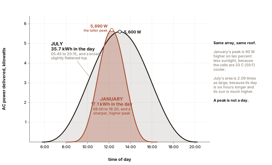
A 7.04 kilowatt array will deliver 5,600 watts at noon in July and 5,690 watts at noon in January, and 35.7 kilowatt-hours on the July day against 17.1 on the January one. This chapter derives every one of those numbers, and then works out what they are worth.
Everything up to here has been about one panel or one component. This chapter is the assembly, and it is the chapter the book’s subtitle promised: the arithmetic that takes a nameplate and produces the number of kilowatt-hours a roof will actually deliver, along with a price.
The method has five steps and none of them is difficult.
- How much sunlight lands on the plane of the array, per day, per month, per year.
- How much of it the array converts, from the nameplate.
- What the losses take, compounded honestly.
- What the result is worth, from the tariff.
- Whether that beats what it cost, including the case where it does not.
Start with a measurement, because the first step is the one people take from a website and never check.
ON THE BENCH: Five tilt angles, one day
Parts: one panel, 10 to 100 W; a plank and some blocks, or a cheap adjustable stand; a protractor or a phone with an inclinometer app; a multimeter on its current range; a compass or the sun itself. Cost: nothing beyond earlier boxes. Time: one clear day, a reading every hour. Hazards: none. Method: aim the panel toward the equator, south in the northern hemisphere. Measure short-circuit current, not power, because Chapter 4 established that short-circuit current is proportional to the sunlight arriving in the plane of the panel and is almost unaffected by temperature. That makes your panel an irradiance meter and removes the biggest confounder in one stroke. At each hour, take five readings in quick succession at tilts of 0, 20, 35, 50 and 90 degrees, and record all five plus the time. What you should see: at noon, the 35 degree reading highest at mid-latitudes, with 20 and 50 within a few percent of it, flat losing about a tenth, and vertical losing a quarter. The spread between 20 and 50 degrees will be far smaller than you expect, which is the practical result of this whole exercise. Then add the day up. Sum each tilt’s hourly readings across the whole day. The daily totals rank differently from the noon readings, because a shallow tilt catches more of the early and late sun while a steep one catches more at noon. The tilt that wins at noon is not always the tilt that wins over the day, and that distinction is what the tables in Section 2 are really encoding. If you can extend it: repeat the same day’s work in three different months. The optimum tilt moves by roughly the change in the sun’s noon elevation, which is 47 degrees between the solstices, and seeing that with your own panel makes Section 3 obvious rather than abstract.
Section 1: Peak Sun Hours
Sunlight is measured as energy per unit area per day, in kilowatt-hours per square metre per day. A good clear site at mid-latitudes averages between 3.5 and 5.5 of those over a year.
That unit converts into something more useful by a trick so convenient it feels like cheating. Since standard test conditions are 1,000 W/m², which is 1 kW/m², a day that delivers 4.5 kWh/m² is a day equivalent to 4.5 hours at exactly standard test conditions. So:
peak sun hours per day = kWh/m² per daySame number, different name. And peak sun hours multiplied by nameplate kilowatts gives nameplate kilowatt-hours, which is the starting point of every estimate.
For the site in this book, a house at 40 degrees north with its array at 35 degrees tilt facing due south, the figures are:
| Period | Peak sun hours per day |
|---|---|
| Annual average | 4.5 |
| July | 6.5 |
| January | 2.7 |
| April and September, roughly | 4.8 |
Note the ratio between July and January: 2.4 to 1. Not the ten to one that the difference in day length and sun angle might suggest, because the January figure is measured on a tilted plane, and a tilted plane catches the low winter sun much better than the ground does. That is the whole reason arrays are tilted, and Section 2 quantifies it.
Where do these numbers come from? Long-run satellite and ground records, published free by national meteorological services and by tools that interpolate them. This is the one input in the whole calculation that you should take from data rather than derive, because it encodes decades of local cloud behaviour that no formula reproduces. What you can and should do is check the tool’s figure against your own measurements, which is what the last bench box in this chapter is for.
Section 2: Tilt and Azimuth, and How Little They Matter
Here is the table that surprises everybody, expressed as a percentage of the best achievable annual yield at 40 degrees north.
| Tilt | Facing south | 45 degrees off south | Due east or west | Due north |
|---|---|---|---|---|
| 0 degrees, flat | 89 | 89 | 89 | 89 |
| 20 degrees | 97 | 95 | 88 | 74 |
| 35 degrees, optimum | 100 | 96 | 82 | 58 |
| 50 degrees | 98 | 94 | 78 | 49 |
| 90 degrees, vertical | 74 | 70 | 56 | 28 |
Read the second and third rows and the practical conclusions fall out.
Getting the tilt wrong costs almost nothing. Anything between 20 and 50 degrees is within three percent of optimum. Nobody should re-roof a house or build a tilted frame on a flat roof to chase that.
Getting the direction wrong costs less than people fear. A roof facing 45 degrees away from the equator, which is to say southeast or southwest at 40 degrees north, gives 96 percent. Four percent. That is one module out of twenty-five, and it is far cheaper to add a module than to argue with a roof.
A shallow pitch forgives a bad direction. Look down the columns: at 20 degrees of tilt, the east-west penalty is 9 percent; at 50 degrees it is 20 percent. A nearly flat array barely knows which way it points, because it is looking mostly at the sky rather than at the sun.
East and west are usable, and north is not. An east or west roof at a shallow pitch delivers 88 percent, which makes it entirely worth covering. A north-facing plane at 40 degrees north delivers 58 percent at optimum tilt and less as the pitch steepens, and it is almost never worth the racking.
And a due-east and due-west pair has a virtue the table hides. Two arrays facing opposite ways produce a broad, flat curve across the day instead of a single midday spike. Under a tariff that pays little for midday export, as Chapter 11 described, that flatter shape can be worth more than the four percent of annual energy it gives up, because more of it is consumed in the house rather than exported. It also clips far less, so it tolerates a higher DC to AC ratio.
IN PLAIN ENGLISH: People agonise over which way their roof faces and at what angle, and mostly they should not. Anything from southeast through south to southwest, at any normal roof pitch, is within a few percent of perfect. Facing due east or west costs you about a tenth. Only a north-facing roof is a real problem. If the answer to your roof’s orientation is “not ideal”, the fix is usually one more panel, not a different house.
Section 3: The January Problem
The annual total conceals the thing that decides whether an array can carry a household, so look at the shape rather than the total.
At 40 degrees north, July delivers 6.5 peak sun hours a day and January delivers 2.7. Add the temperature effect, which runs the other way, and the difference in output is smaller than the difference in sunshine but still large.
Non-temperature losses multiply to 0.868, from Section 4’s table.
July, at an average generating-hour cell temperature of 55 °C (131
°F), so a temperature factor of 1 - 0.0034 x 30 = 0.898:
7.04 x 6.5 x 0.868 x 0.898 = 35.7 kWh in the day
January, at an average generating-hour cell temperature of 15 °C (59
°F), so a factor of 1 + 0.0034 x 10 = 1.034:
7.04 x 2.7 x 0.868 x 1.034 = 17.1 kWh in the day
35.7 kilowatt-hours against 17.1. A ratio of 2.09, from a sunshine ratio of 2.4, and the difference between those two ratios is entirely the temperature: the January array is 13 percent more efficient than the July one, per unit of sunlight received.
Now the instantaneous figures, which are the ones the book’s opening promise named.
Noon in July. Full sun at 1,000 W/m², air at 32 °C (90 °F), so by Chapter 9’s formula the cells are at 63 °C (145 °F):
7,040 x 1.00 x (1 - 0.0034 x 38) = 6,130 W at the modules
x 0.98 soiling x 0.98 mismatch x 0.98 wiring = 5,770 W into the inverter
x 0.97 inverter = 5,600 W of AC
Noon in January. A clear winter day at 40 degrees north puts about 900 W/m² on a 35 degree plane, because the sun is nearly square to it even though it is low in the sky. Air at 2 °C (36 °F), so the cells reach 30 °C (86 °F):
7,040 x 0.90 x (1 - 0.0034 x 5) = 6,228 W at the modules
x 0.9412 = 5,862 W into the inverter
x 0.97 = 5,690 W of AC
The January noon figure is higher than the July one. 5,690 W against 5,600 W, on ten percent less sunlight, because the panels are 33 °C (59 °F) cooler.
That is the counterintuitive result this book has been building toward since Chapter 1, and it arrives not as an assertion but as the output of six lines of arithmetic using two numbers off a datasheet. The best instantaneous output a domestic array ever produces is on a cold clear day, not a hot one. Ask anyone with a monitoring app and they will confirm that their record peak was in winter or early spring, and most of them have no idea why.
And yet January produces less than half the energy of July, because a peak is not a day. The January sun rises late, sets early, and spends most of its short arc at a low angle. Peak power and daily energy are two different questions with two different answers, and a great deal of confusion about solar comes from conflating them.
Section 4: The Derate Chain, Compounded Honestly
Now the full annual calculation, and the discipline is to list every loss, give each a defensible number, and multiply rather than add.
| Loss | Multiplier | Why |
|---|---|---|
| Soiling | 0.98 | dust and pollen between rains |
| Shading | 0.97 | one chimney, morning only |
| Module mismatch | 0.98 | modules are not identical |
| DC wiring | 0.98 | Chapter 10’s I²R |
| Inverter conversion | 0.97 | Chapter 11’s weighted efficiency |
| Cell temperature, annual average | 0.94 | Chapter 9 |
| Availability and downtime | 0.995 | outages, faults, maintenance |
| Nameplate tolerance and first-year losses | 0.985 | binning and light-induced degradation |
0.98 x 0.97 x 0.98 x 0.98 x 0.97 x 0.94 x 0.995 x 0.985 = 0.816
A performance ratio of 0.816. Which is to say the array delivers about 82 percent of the energy that its nameplate and the local sunshine would suggest, and that figure is typical of a well-built system. Anything above 0.85 is exceptional and anything below 0.75 has a problem worth finding.
Then the annual energy:
7.04 kW x 4.5 peak sun hours x 365 days x 0.816 = 9,435 kWh
Call it 9,400 kWh a year, which is 1,340 kilowatt-hours for every kilowatt installed, and that specific-yield figure is the one to quote when comparing sites, because it strips out system size entirely.
Two honesty notes about this table, because a derate chain is easy to fudge.
The instantaneous calculations in Section 3 used only three of these multipliers, not eight. Soiling, mismatch and wiring apply at any moment. Shading, availability and nameplate tolerance are annual averages and do not belong in a calculation for a specific clean, clear, working noon. Mixing the two is the commonest error in this arithmetic and it double-counts several percent.
And the temperature multiplier of 0.94 is a whole year’s average, not a measurement. It is defensible for a temperate site and it is wrong for Phoenix, where 0.90 is nearer, and wrong for Edinburgh, where 0.97 is nearer. If you change nothing else in this table for your own site, change that one, because it is the only entry that varies strongly with climate.
Section 5: The Roof, End to End
Now design the thing.
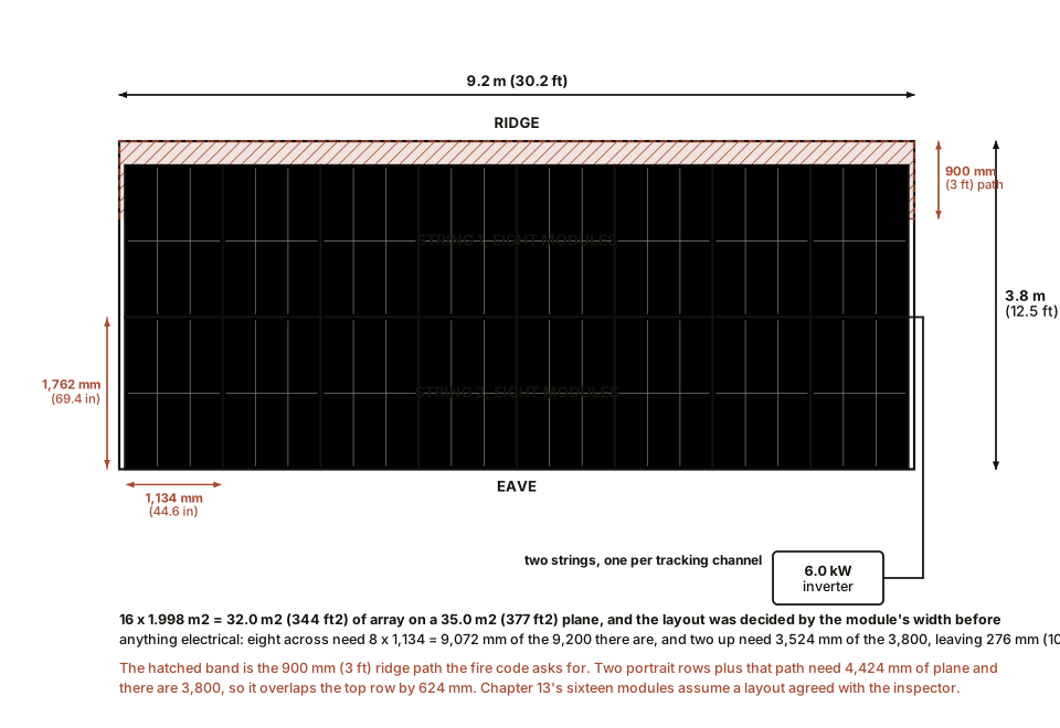
The roof. A south-facing plane at 30 degrees pitch, 9.2 m wide and 4.5 m from eave to ridge, which is 30.2 by 14.8 ft, so 41.4 m² (446 ft²) of surface. Local fire code wants a 900 mm (3 ft) clear path at the ridge, so the usable height is nearer 2.9 m (9.5 ft) unless the array is set to one side. Assume a layout agreed with the inspector that permits two rows.
The module. 440 W, 1,762 by 1,134 mm (69.4 by 44.6 in), so 1.998 m² (21.5 ft²) each, at 22.0 percent efficiency, weighing 21.0 kg (46.3 lb).
The layout. Portrait orientation, 1.134 m (44.6 in) of width each, so 8 across the 9.2 m width with a little to spare. Check the other direction, because this is where roof plans usually fail: two portrait rows are 3.524 m (11.6 ft), the ridge path takes 900 mm (3 ft), and 3.524 plus 0.9 is 4.424 m (14.5 ft) against the 4.5 m (14.8 ft) available. It fits, with 76 mm (3 in) to spare. Two rows of 8 gives 16 modules, 7.04 kW, occupying 32.0 m² (344 ft²) of the 41.4 m² plane.
The strings. One row per string, 8 modules each, into the inverter’s two tracking channels. Chapter 10 already checked both ends of the temperature range: 340 V open circuit on the coldest morning, under the 600 V residential limit, and about 220 V at the maximum power point on the hottest afternoon, well above the inverter’s 125 V lower tracking limit.
The inverter. 6.0 kW AC, DC to AC ratio 1.17, which Chapter 11 showed clips only about 0.3 percent of annual output.
Structural load. Sixteen modules at 21.0 kg is 336 kg (741 lb) of module plus perhaps 90 kg (198 lb) of rail and clamps, so 426 kg (939 lb) spread over 32.0 m² (344 ft²). That is 13.3 kg/m², or 2.7 lb/ft², which any roof built to carry snow will accept without modification. Wind uplift is the real structural question, not weight, and it is set by the fixing pattern and the local code rather than by anything in this book.
The bill of materials, self-installed:
| Item | Cost |
|---|---|
| 16 modules at $135 | $2,160 |
| 6.0 kW inverter | $1,250 |
| Rails, clamps, flashings, roof hooks | $900 |
| PV wire, conduit, MC4 connectors, DC and AC disconnects, rapid-shutdown devices | $700 |
| Permit and inspection | $500 |
| Tools, fall protection, consumables, mistakes | $1,000 |
| Total | $6,510 |
$6,510 / 7,040 W = $0.92 per watt
And the same system installed professionally at a typical turnkey rate of $2.90 per watt:
7,040 x $2.90 = $20,400, or $14,280 after a 30 percent tax credit
A factor of two to three, for the same hardware on the same roof. Chapter 3’s learning-curve arithmetic predicted exactly this: the modules are on a manufacturing curve and the labour and paperwork are not. The modules are 33 percent of the self-installed cost and 11 percent of the professional one.
Whether self-installation is available to you depends on your jurisdiction, your roof, your competence with a fall-arrest harness, and whether your utility will connect a system it did not watch being built. This book is not going to tell you to go on a roof. It will tell you plainly that the price difference is a labour and permitting difference rather than a quality difference, because a reader deciding on twenty thousand dollars deserves to know where the money goes.
Section 6: What It Is Worth, Four Ways
Now Step 4, and this is where a single answer would be a lie. Take the 9,400 kWh a year and apply Chapter 11’s value formula under four real tariff regimes.
| Tariff situation | Value per kWh | Annual value | Payback, self-installed at $6,510 | Payback, professional at $14,280 |
|---|---|---|---|---|
| Net metering, retail $0.32 | $0.320 | $3,008 | 2.2 years | 4.7 years |
| Net metering, retail $0.16 | $0.160 | $1,504 | 4.3 years | 9.5 years |
| Net metering, retail $0.11 | $0.110 | $1,034 | 6.3 years | 13.8 years |
| Net billing, $0.16 retail and $0.05 export, 40 percent self-consumed | $0.094 | $883 | 7.4 years | 16.2 years |
Between 2.2 and 16.2 years, from the same array in the same sunshine. Nothing about the hardware differs across those four rows. The entire spread is tariff and labour.
Five things change these numbers and all five should be in an honest calculation.
Degradation. Chapter 14’s 0.5 percent a year means output averages about 94 percent of year one across 25 years, so a lifetime total near 220,000 kWh rather than 235,000. It lengthens every payback by roughly 6 percent.
Inverter replacement. Expect one, at year 12 to 15, for about $1,250 in today’s money. Add it.
Electricity price inflation. Retail rates have historically risen faster than general inflation in most markets, which shortens payback. This is the term most often abused in sales material, because assuming five percent annual escalation for twenty-five years roughly halves the apparent payback and is not defensible. Run the calculation at zero escalation, and treat anything better as a bonus.
The cost of capital. A payback period ignores it entirely, which is why payback is a poor measure. A system with a twelve-year simple payback, financed at seven percent over twenty years, may never pay back at all, because the interest alone exceeds the savings for the first decade. If borrowing, compare the loan payment against the bill reduction month by month, and if the loan payment is larger, the project loses money from day one however good the physics.
And the roof’s remaining life. An array outlives a roof covering. If the roof needs replacing within ten years, replace it first, because removing and refitting sixteen modules costs $2,000 to $4,000 and is entirely avoidable.
Put the whole thing on the honest footing, which is levelised cost rather than payback:
self-installed: ($6,510 + $1,250) / 220,000 kWh = $0.035 per kWh
professional: ($14,280 + $1,250) / 220,000 kWh = $0.071 per kWh
professional, no credit: ($20,400 + $1,250) / 220,000 = $0.098 per kWh
Three and a half cents a kilowatt-hour self-installed; seven to ten cents professionally. Against a retail rate of eleven to thirty-two cents. On a levelised basis solar wins nearly everywhere, and it can still be a bad investment for a particular household, because levelised cost ignores when the money is spent, whether the energy arrives when it is needed, and what the alternative use of the capital was. Both statements are true and a reader should hold both.
Section 7: The Same Design, on the Ground
Take the identical sixteen modules and put them on a ground-mounted frame in the garden instead.
What improves:
Tilt is chosen rather than inherited. 35 degrees instead of the roof’s 30, worth about 1 percent.
Cooling is much better. An open rack with air on all sides runs cooler than a roof array on standoffs, and the effective operating temperature drops by 5 to 8 °C (9 to 14 °F). At 0.34 percent per degree that is 2 to 3 percent of annual output recovered.
Cleaning and maintenance are trivial. You can hose the array down and you can reach a failed connector without a harness. Soiling improves from 0.98 to 0.99.
And nothing is bolted through your roof. Sixty-four penetrations through a waterproof surface is sixty-four opportunities for a leak in twenty-five years, and the ground mount has none.
Total gain: about 5 percent, so 9,900 kWh instead of 9,400.
What it costs:
| Item | Extra cost |
|---|---|
| Ground-mount frame, posts and concrete instead of roof rails | $1,600 |
| Trenching, conduit and a longer cable run | $900 |
| Total extra | $2,500 |
extra output 500 kWh a year, at $0.16 = $80 a year
$2,500 / $80 = 31 years
Thirty-one years to recover the difference, on a 25-year array. So the ground mount is technically better and economically worse, and the conclusion is not that ground mounts are wrong but that the reason to build one is never the extra five percent.
The reasons to build one are: the roof faces north, the roof is shaded, the roof is too old, the roof is too small, the roof is not yours, or you would rather not drill sixty-four holes in it. Any of those is sufficient and the yield is a side benefit. Which is the general shape of good engineering decisions: the number that justifies a choice is rarely the number that first attracted you to it.
ON THE BENCH: Log a week, then check your own prediction
Parts: one panel; a logging DC energy meter with a shunt, about $25, or a data-logging multimeter; a resistive load near the panel’s maximum power point; a notebook. Cost: about $25. Time: set up in an hour, then leave it a week. Hazards: none. Weatherproof the meter or bring it in each evening. Method: before you start, predict. Look up your site’s peak sun hours for the month, apply the derate chain from Section 4 with the temperature multiplier adjusted for your climate, and write down the kilowatt-hours you expect for each of the next seven days. Seal the prediction in an envelope if you want to be honest with yourself. Then log the week. What you should find: your total for the week within perhaps 15 percent of the prediction, and the individual days scattered much more widely because of cloud. The week matches better than any single day does, which is the whole reason solar output is quoted monthly and annually rather than daily. Then find your errors. If you are consistently high, suspect your assumed peak sun hours, or a fixed load that is not sitting at the maximum power point. If you are consistently low, suspect soiling, or a shadow you have not noticed, or a panel hotter than you assumed. Go and measure the thing you suspect rather than adjusting the model to fit. The most valuable outcome: knowing the size of your own uncertainty. A reader who can say “my estimate is good to about 12 percent and here is why” is in a far stronger position than one quoting a website’s figure to four significant digits.
SLOW DOWN. Check Your Understanding: A household uses 9,400 kWh a year. An installer proposes exactly the array in this chapter, 7.04 kW producing 9,400 kWh a year, and describes it as covering 100 percent of their electricity. Under one-for-one net metering that description is fair. Under net billing with a $0.05 export credit, what fraction of their bill does it actually cover, and why is the answer so much worse than 100 percent? Answer before reading on.
Roughly 55 to 60 percent of the bill, not 100 percent.
The array produces 9,400 kWh and the house uses 9,400 kWh, but not at the same times. Take the 40 percent overlap assumed earlier: 3,760 kWh is consumed as it is generated, saving the full $0.16, which is $602. The other 5,640 kWh is exported at $0.05, earning $282. Total value $883.
Meanwhile the house still imports 5,640 kWh from the grid, at $0.16, which is $902. The bill did not go to zero; it went from $1,504 to about $620 of energy charges, plus whatever fixed connection charge the utility levies regardless. And that fixed charge is now a much larger share of a much smaller bill.
Three things follow, and they are the practical end of this chapter.
“Covers 100 percent of your usage” and “eliminates your bill” are different claims, and only the first one is being made. Ask which.
Under net billing, the useful array is smaller than the annual-usage match. Sizing to the household’s daytime consumption rather than its annual total gives a better return per dollar, because the last modules produce almost purely export-rate energy. That is the opposite of the advice that was correct under net metering, and it is why old rules of thumb mislead.
And the fixed connection charge is untouchable by any array. In some markets it is $10 a month and in others $40, and a household paying $40 has a floor of $480 a year that no amount of solar will reduce. It belongs in the payback calculation, and it is almost never in the quotation.
Chapter 14 asks what goes wrong over the twenty-five years this chapter’s arithmetic just assumed.

Bench Degree
Get the degree without the diploma.
Learn the material, not how to pass the exam.