Bench Degree·SOLAR POWERchapter

Chapter 9: Temperature, Shade and the Real Output
Take a panel out of the freezer into the sun and it will read higher than its nameplate. Play a hairdryer over the same panel and it will read a fifth lower. The desert is not the best place for solar power, and this chapter is where you find that out with a hairdryer.
Do this one indoors first, with a small panel, and it will change how you think about the subject.
Put the panel in a chest freezer or a domestic freezer compartment for half an hour, wrapped in a plastic bag so it does not frost up. While it is in there, set up a bright lamp, or better, arrange to carry the panel outside quickly. Measure open-circuit voltage the moment you take it out, then every fifteen seconds as it warms.
Then, separately, put the panel in the sun and play a hairdryer over its face on a low setting, watching the voltage.
Here is what the 100 W panel from Chapter 1 does. Its nameplate open-circuit voltage is 22.0 V at 25 °C (77 °F), and its temperature coefficient of voltage is 0.36 percent for every degree Celsius, which is 0.20 percent for every degree Fahrenheit, or 79 millivolts per degree Celsius.
| Panel temperature | Predicted Voc |
|---|---|
| −5 °C (23 °F) | 24.4 V |
| 5 °C (41 °F) | 23.6 V |
| 25 °C (77 °F) | 22.0 V |
| 45 °C (113 °F) | 20.4 V |
| 65 °C (149 °F) | 18.8 V |
Five and a half volts of range on a panel described as a 22 volt panel. Not a small effect, not a second-order correction, and entirely predictable from one number on the datasheet.
ON THE BENCH: Measure your panel’s temperature coefficient
Parts: a small panel, 10 to 50 W; a freezer; a hairdryer; a thermocouple thermometer or an infrared thermometer, about $20; a multimeter; a plastic bag; masking tape. Cost: about $20 if you own the meter. Time: 90 minutes. Hazards: do not exceed about 80 °C (176 °F) on the panel; the encapsulant softens above that and the panel is not designed for a hairdryer on high held close. Keep the dryer moving and off the highest setting. Do not get water on a cold panel and then heat it. Method: you must hold the light constant while changing the temperature, so work with open-circuit voltage rather than power, and work indoors under a fixed lamp or on an overcast day when irradiance is steady. Tape the thermocouple to the back of the panel. Record voltage and temperature together, in pairs, from the freezer all the way up to hairdryer-hot, as many pairs as patience allows. Then plot Voc against temperature and take the slope, in volts per degree Celsius and volts per degree Fahrenheit. Divide by the nameplate Voc to get percent per degree. What you should get: between 0.30 and 0.40 percent per degree Celsius, which is 0.17 to 0.22 percent per degree Fahrenheit. Compare against the datasheet. Most readers find agreement within about ten percent, which for a kitchen measurement of a semiconductor property is very good indeed. If the line is not straight: check that the light really is constant. A cloud thinning during the run will bend the line and you will blame the physics. Why open circuit and not power: power depends on both temperature and light, and you cannot hold light constant well enough by hand to separate them. Voc depends on light only through a logarithm, as Chapter 6 showed, so a ten percent drift in irradiance moves it by six millivolts and you can ignore it. Choosing the measurement that is insensitive to what you cannot control is the whole craft of benchwork.
Section 1: Three Coefficients, and Which One Matters
Every module datasheet lists three temperature coefficients, and they do not all point the same way.
| Quantity | Coefficient, cheap panel | Coefficient, good modern module |
|---|---|---|
| Power at maximum power point | −0.42 percent per °C | −0.34 percent per °C |
| Open-circuit voltage | −0.36 percent per °C | −0.27 percent per °C |
| Short-circuit current | +0.05 percent per °C | +0.045 percent per °C |
Current goes up with temperature. A warmer semiconductor has a very slightly narrower band gap, so a few more of the long-wavelength photons make it across the threshold. The effect is real and it is tiny.
Voltage goes down, substantially, for the reason
Chapter 6 gave: the cell’s reverse saturation current roughly doubles
for every 10 °C (18 °F) of temperature rise, which shrinks the logarithm
that sets Voc.
Power goes down slightly faster than voltage, because the fill factor sags a little as well.
The power coefficient is the one that costs you money, and the conversion is worth keeping in your head: for a module at −0.34 percent per degree Celsius, that is −0.19 percent per degree Fahrenheit. So a panel 40 °C (72 °F) above standard test conditions has lost 13.6 percent of its output.
IN PLAIN ENGLISH: A hot solar panel makes less electricity than a cold one from the same sunlight. Not a little less. Something like a sixth less on a hot summer afternoon. The panel is not broken and it is not dirty; it is simply hot, and hot is the condition it works worst in. Which means the mental picture almost everybody has, of solar power belonging in a blazing desert, has the temperature part exactly backwards. Bright and cold is the ideal, and bright and cold is what a clear day in early spring is.
Section 2: How Hot Does a Panel Actually Get
The datasheet number is useless without knowing the temperature the panel will reach, and it reaches far more than the air temperature. A panel in full sun absorbs about 80 percent of the sunlight landing on it, as Chapter 8’s ledger showed, and it has to get rid of nearly all of that as heat.
The industry’s estimate is built on one measured figure. NOCT, the nominal operating cell temperature, is the temperature a module reaches in 800 W/m² of sunlight, 20 °C (68 °F) air, and a 1 m/s (2.2 mph) breeze, open circuit, mounted with air behind it. For a modern module it is around 45 °C (113 °F); for a cheap one, 47 °C (117 °F).
Read that again: 20 °C (68 °F) air produces a 45 °C (113 °F) panel. Twenty-five degrees Celsius of rise, forty-five degrees Fahrenheit, in a light breeze at four fifths of full sun.
From NOCT you can estimate cell temperature at any condition:
Tcell = Tair + ((NOCT - 20) / 800) x irradianceWork it for a summer afternoon, air at 32 °C (90 °F), full sun at 1,000 W/m², with a module of NOCT 45:
Tcell = 32 + (25 / 800) x 1,000 = 32 + 31 = 63 °C
63 °C, which is 145 °F. That is 38 degrees Celsius above standard test conditions, and at −0.34 percent per degree it is a loss of 12.9 percent before anything else has gone wrong.
Three practical consequences fall out of that formula.
Mounting matters, a lot. The formula assumes open-back mounting with air circulating. A module laid flush against a roof surface, or built into the roof as a tile, runs 5 to 15 °C (9 to 27 °F) hotter than one on standoffs with a 100 mm (4 in) air gap, and pays for it in output all summer. A ground-mounted array is measurably better than a roof array for this reason alone, typically by 2 to 4 percent of annual yield.
Wind is worth real money. The same array on a breezy site runs cooler and produces more. This is not a small term and it is one of the reasons two identical systems in the same town can differ by several percent.
And the loss is worst exactly when the grid needs the power most. A hot still afternoon in July is the peak of air-conditioning demand and it is also when the array is 13 percent down. That mismatch is a real cost to a utility and it is part of why storage became interesting.
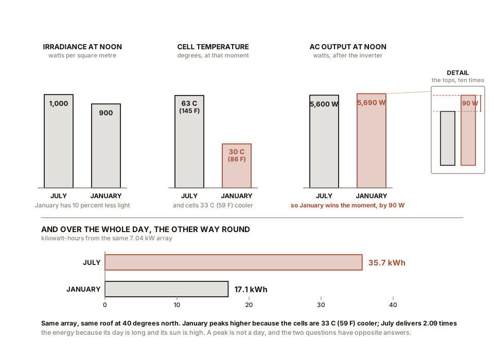
Section 3: Separating the Two Effects on One Day
Here is the measurement that makes all of this concrete, and it needs nothing but a panel, a load, a meter and a thermometer over the course of one day.
Take the Chapter 1 panel and read it twice.
At 7 a.m.: irradiance 200 W/m², panel temperature 18 °C (64 °F).
100 W x (200/1,000) x (1 + 0.0042 x 7) = 20 x 1.029 = 20.6 W
At 2 p.m.: irradiance 950 W/m², air 33 °C, panel temperature 65 °C (149 °F).
100 W x (950/1,000) x (1 - 0.0042 x 40) = 95 x 0.832 = 79.0 W
Now the trick that separates the two effects. Divide each output by its own irradiance, which removes the sunlight and leaves only the temperature:
morning: 20.6 / 0.200 = 103
afternoon: 79.0 / 0.950 = 83
The panel is 19 percent less efficient in the afternoon than at dawn, and the entire difference is temperature. Check it against the coefficient: the panel was 47 degrees Celsius hotter, at 0.42 percent each, which is 19.7 percent. The prediction and the measurement agree to within a rounding error.
That is the whole method, and it works on any array on any day. Normalise output by irradiance and what remains is the temperature story, cleanly separated. It is also how you tell a temperature problem from a shading problem from a dirt problem in the field, which Chapter 14 turns into a procedure.
ON THE BENCH: One day, one panel, two effects separated
Parts: a panel; a fixed resistor near the panel’s maximum power point value; two multimeters, or a cheap logging wattmeter; an irradiance meter or reference cell; a thermocouple taped to the panel’s back. Cost: nothing beyond earlier boxes. Time: a full clear day, with a reading every half hour. Hazards: none. Wear a hat. Method: fix the panel at a tilt roughly equal to your latitude, facing the equator, and do not move it all day. Every thirty minutes record time, irradiance, panel back temperature, voltage and current. Then make three plots: output against time, which is the shape everybody expects; irradiance against time; and output divided by irradiance against time, which is the plot almost nobody makes. What you should see: the first two plots roughly symmetrical about solar noon. The third one sloping downhill all day, from a high point in the morning to a low point in mid-afternoon, and recovering slightly toward evening. That downhill slope is the panel heating up, isolated from everything else. The number to extract: the ratio between your best morning point and your worst afternoon point, divided by the temperature difference between them. It should come out near your panel’s power temperature coefficient. You have measured a semiconductor property using the sun as the instrument.
Section 4: One Cell, Most of the Output
Now the other half of this chapter, which is the shading demonstration you already did in Chapter 1 with a thumb.
Series-wired cells carry the same current. All of it, through every one of them, in turn. So the current through a string is set by the worst cell in it, in exactly the way the flow through a hosepipe is set by its narrowest point regardless of how wide the rest is.
Shade one cell to a tenth of full light and it can pass only a tenth of the current. Every other cell in that string is now throttled to a tenth as well, whatever the sun is doing to them. One cell in thirty-six, and the panel loses ninety percent.
Worse than merely losing it. The other thirty-five cells are still generating voltage and still trying to push current through the shaded one, which is refusing to pass it. So the shaded cell is driven backwards, into reverse bias, and it starts absorbing power rather than producing it.
Put a number on that, because it is what destroys panels.
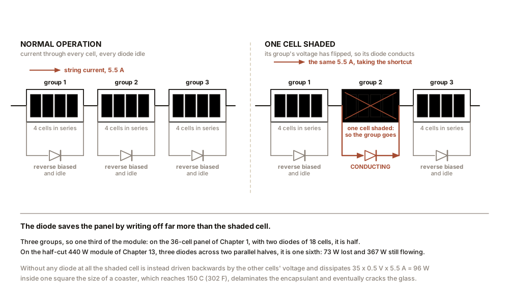
In a 36-cell panel with no protection, a single fully shaded cell can
be reverse biased by roughly the forward voltage of the other 35, so
about 35 x 0.5 = 17.5 V, while carrying the string current
of 5.5 A.
17.5 x 5.5 = 96 W
Ninety-six watts, dissipated inside one cell the size of a coaster. A panel rated at 100 W is now a 96 W heater concentrated into one small square. That is a hot spot, it reaches 150 °C (302 °F) and beyond, and it delaminates the encapsulant, browns the backsheet and eventually cracks the glass. Permanent damage from a leaf.
Section 5: Bypass Diodes, and What They Cost
The fix has been standard since the 1980s and it is three diodes.
A bypass diode is wired across a group of cells, backwards, so that in normal operation it is reverse biased and does nothing at all. When one cell in its group is driven into reverse bias, the voltage across the group flips, the diode conducts, and the string current takes the diode as a shortcut around the whole group.
Which does two good things and one bad thing.
Good: the shaded cell is no longer forced to dissipate the string’s power, so the hot spot is prevented. Good: the rest of the string keeps working, because current can still flow.
Bad: the entire group is out of the circuit, not just the shaded cell.
Work out what that costs on the two panels in this book.
The Chapter 1 panel, 36 cells, two bypass diodes at 18 cells each. Shade one cell and its group of 18 is bypassed. Output falls from 100 W to about 50 W, and the panel loses half its production to one shaded cell. Cheap 100 W panels frequently have no bypass diodes at all, in which case the output collapses to almost nothing, which is exactly the range Chapter 1 predicted for the thumb experiment: 50 percent with diodes, 90 percent or more without.
The 440 W module of Chapter 13, 108 half-cut cells, three bypass diodes. Here the architecture is cleverer. The cells were cut in half at manufacture and wired as two independent halves in parallel, with three diodes spanning three groups. Shade one half-cell and you bypass one group in one half, which is one sixth of the module: about 73 W lost out of 440, and 367 W still flowing.
That is the reason half-cut cells took over the
industry, and it is not the reason usually given. The usual
explanation is lower resistive losses, since halving a cell halves its
current and quarters its I²R loss, and that is true and
worth about 2 percent. The shade tolerance is worth far more
than that on any real roof, and it costs nothing extra, because
the cells were going to be cut anyway.
ON THE BENCH: Find the diodes, then confirm what they do
Parts: a panel whose junction box you can open, or a junction box from a scrapped panel, free from any installer; a multimeter with a diode test function; a piece of card. Cost: nothing. Time: 45 minutes. Hazards: open the junction box only on a panel that is face down or covered, so it is producing nothing. A 440 W module in sun has 38 V across those terminals and will deliver 14 A into a slipped screwdriver. Method: with the panel covered, unclip the junction box lid. You will find the ribbons from the cell strings and, bridging them, two or three small black packages, each with a heatsink tab. Those are the bypass diodes. Use the meter’s diode function to confirm each conducts one way and not the other, and note which pairs of ribbons each one bridges. Sketch it. That sketch is the panel’s internal wiring, and you have obtained it without breaking anything. Then, in the sun, with the box closed: load the panel at its maximum power point and record output. Cover exactly one cell with card and record again. Move the card to a cell in a different group and record again. Then cover one cell in each group at once. What you should see: one shaded cell taking out a predictable fraction, a half or a third or a sixth, that matches the diode count you sketched. And shading one cell in every group at once takes out nearly everything, because there is no group left to carry the current. The number worth having: shading exactly one cell in a column across the panel usually costs far more than shading a whole row, or vice versa, depending on how the strings snake. Which direction hurts more tells you which way to prune the tree, and it is the single most useful piece of shade diagnosis you can do on a real installation.
Section 6: Three Architectures, on the Merits
If shading is the problem, there are three ways to build an array and they differ in what shade costs. Take the 7.04 kW array of sixteen modules from Chapter 13 and price each.
String inverter. All sixteen modules in two series strings of eight, both feeding one inverter with two tracking channels. About $1,250. One tracker per string of eight, so the tracker finds a single operating point for eight modules and any module that cannot deliver at that point drags on the rest. Simple, one device, one thing to fail, and the cheapest by a wide margin.
DC optimisers. A small converter bolted to each module, presenting each one with its own maximum power point and passing the result to a string inverter. About $960 for sixteen, plus a compatible string inverter, so around $2,210. Every module works at its own best point. Sixteen extra electronic devices, on a roof, in the weather, at panel temperature.
Microinverters. A complete small inverter per module, producing mains-voltage AC on the roof. About $2,400 for sixteen, and no string inverter at all. Per-module tracking, no high-voltage DC anywhere on the building, and per-module monitoring that tells you which panel is failing. Sixteen devices again, and again on the hot side of the roof.
What the module-level options buy, honestly:
| Roof condition | Gain from module-level electronics |
|---|---|
| No shade at all, one plane, one orientation | 0 to 2 percent |
| Light morning or evening shade from a distant tree | 3 to 8 percent |
| A chimney, a vent stack, or a real tree over part of the array | 8 to 25 percent |
| Multiple roof planes at different orientations | 5 to 15 percent |
On an unshaded single-plane roof, module-level electronics are close to a waste of money. The extra $1,000 buys perhaps 1 percent of 9,400 kWh a year, which is 94 kWh, which at $0.16 is $15 a year. That is a sixty-six year payback on a component with a twenty-five year warranty.
On a shaded roof they are the difference between a good system and a bad one, and the same $1,000 buying 15 percent returns $225 a year and pays back in under five.
The reliability comparison is genuinely contested and worth flagging as such. Module-level electronics multiply the device count by sixteen and put every device in the hottest, least accessible place available, which argues one way. Against that, microinverter manufacturers offer 25-year warranties where string inverter makers typically offer 10 to 12, and a string inverter failure takes the whole array offline while a microinverter failure costs one panel. Field failure-rate data is largely held by manufacturers and installers rather than published independently, so anyone claiming a settled answer is guessing. What would settle it is long-run independent fleet data, and it is slowly appearing.
SLOW DOWN. Check Your Understanding: A homeowner in Phoenix, Arizona and one in Edinburgh, Scotland install identical 7 kW arrays. Phoenix receives roughly twice the annual sunlight that Edinburgh does. Before reading on, decide whether Phoenix produces twice as much, more than twice, or less than twice, and say why.
Less than twice, and by a noticeable margin.
Phoenix gets about twice the irradiation, which is the dominant term and it does win. But its panels spend the year far hotter. An array in Phoenix runs at an average cell temperature perhaps 20 °C (36 °F) above one in Edinburgh across the generating hours, and at 0.34 percent per degree Celsius that is nearly 7 percent of output given away that the Scottish array keeps. Phoenix also loses more to soiling, since dust settles and it rarely rains to wash it off, while Edinburgh’s panels are rinsed weekly by the weather whether the owner likes it or not.
So the ratio comes out nearer 1.8 than 2.0. Not a reversal, and it would be dishonest to pretend the desert loses. But it does mean that comparing two sites on sunlight alone systematically overstates the hot one, by five to ten percent, and that is exactly the size of error that turns a marginal payback calculation into a wrong one.
There is a further twist worth carrying into Chapter 13. Edinburgh’s problem is not temperature, it is January. Its annual total is low because its winter is nearly dark, not because its summer is poor: a clear cold day in Scotland in May is close to the best conditions a solar panel ever sees anywhere. Seasonal distribution, rather than annual total, is what decides whether an array can carry a household, and it is why the January figure appears in this book’s opening promise.
Chapter 10 leaves the panel behind and asks how sixteen of them get wired together, and why the answer is several hundred volts.

Bench Degree
Get the degree without the diploma.
Learn the material, not how to pass the exam.