Bench Degree·WIND POWERchapter

Chapter 16: Capacity Factor and the Grid
A gas plant runs at 55 percent capacity factor and a wind farm at 39, and nearly everybody reads that as the wind farm being worse at its job. The two numbers are measuring different things. One is a decision about the market and the other is a fact about the weather.
The hardest engineering in wind power is not in the rotor. It is in the sixty seconds after a lightning strike takes out a transmission circuit and eight hundred megawatts of offshore wind decides, correctly according to its own settings, to disconnect.
This chapter is about the machine’s relationship with the wire, and it starts with the most abused number in energy.
Section 1: What Capacity Factor Actually Measures
Capacity factor is the energy a machine produced in a period, divided by the energy it would have produced running flat out at nameplate for the whole period.
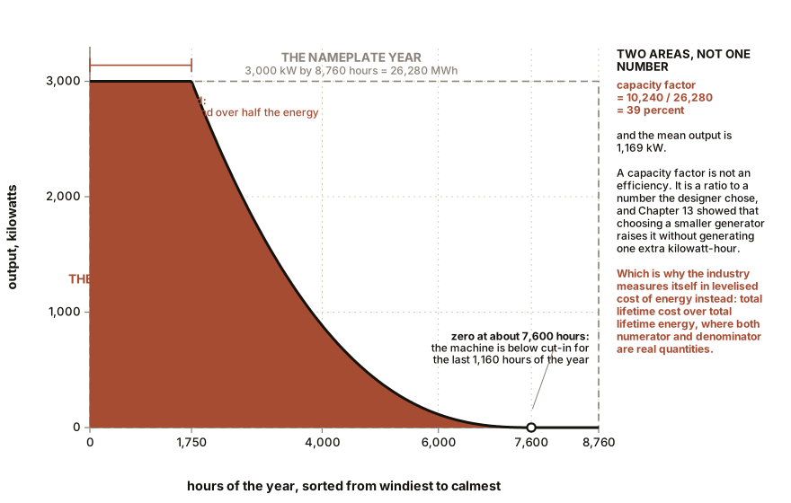
CF = (energy produced) / (nameplate power × hours in the period)For the machine this book has been building: rated 3 MW, at our reference site with a mean wind speed of 7 m/s (16 mph) and a Weibull shape factor of 2. Chapter 13’s power curve, integrated against Chapter 10’s distribution bin by bin, gives an average output of 1,169 kW.
CF = 1,169 / 3,000 = 39 percent
Annual energy = 1.169 MW × 8,760 hours = 10,240 MWh
Ten gigawatt-hours a year from one machine, which at a United States household average of about 10,500 kWh is roughly a thousand homes.
Now here is the composition of that 39 percent, and it is not what most people assume.
| Condition | Share of hours | Share of annual energy |
|---|---|---|
| Below cut-in, producing nothing | 13% | 0% |
| Between cut-in and rated | 67% | 48% |
| At rated power | 20% | 52% |
| Above cut-out | under 1% | 0% |
Read the bold row. The machine sits at its full nameplate output for a fifth of the year, and that fifth delivers more than half of everything it makes. Meanwhile it produces something at all for 86 percent of the hours, which is a number that surprises people who have been told wind is unreliable.
Availability and capacity factor are completely different quantities and conflating them is the commonest error in this subject. Availability is the fraction of time the machine is fit to run, and for a modern onshore turbine it is 97 to 98 percent, comparable with a thermal plant. Capacity factor is the fraction of nameplate it averaged. A turbine can be available all year and still have a capacity factor of 39 percent, and nothing has gone wrong.
Section 2: Why Comparing It To a Gas Plant Is a Category Error
Typical annual capacity factors, and the point is in the third column.
| Plant | Capacity factor | What is limiting it |
|---|---|---|
| Nuclear | 90 to 93% | refuelling and maintenance outages |
| Coal | 40 to 60% | the market: it runs when it is called |
| Combined cycle gas | 50 to 60% | the market: it runs when it is called |
| Onshore wind, older fleet | 25 to 33% | the weather, and the machine’s specific power |
| Onshore wind, new build | 40 to 50% | the weather, and the specific power |
| Offshore wind | 45 to 55% | the weather |
| Rooftop solar, mid latitude | 14 to 18% | the sky, and the night |
Only the first row is close to a technical maximum. A nuclear station runs flat out whenever it is not shut down for refuelling, so its capacity factor genuinely measures reliability.
The coal and gas rows measure nothing about the plant at all. A combined cycle plant is technically capable of about 90 percent, and it does not run at 90 percent because nobody is paying it to. It runs when the price exceeds its fuel cost, which is some of the time. Its capacity factor is a market outcome and it changes every year with the gas price. In a year of cheap gas the same plant reports 70 percent and in a year of expensive gas it reports 30, and no bolt has moved.
And the wind rows measure two things at once, which is what makes the number so slippery. Chapter 13 established that capacity factor depends on the site’s wind distribution and on the machine’s specific power, in unknown proportions unless you are told both. A machine with a bigger rotor on the same generator reports a higher capacity factor while being the same machine in every respect that matters.
So the honest statement is this. Capacity factor is not efficiency, not reliability, not quality and not a score. It is a ratio whose denominator is chosen by a designer and whose numerator depends on the weather. The only fair comparison between two capacity factors is between two machines of similar specific power at sites of known wind resource. Everything else is arithmetic dressed as an argument.
And the number that does mean something, and which the industry actually uses, is the levelised cost of energy: the total lifetime cost of the plant divided by the total lifetime energy it delivers, in dollars per megawatt-hour. That is comparable across technologies, because both its numerator and denominator are real quantities rather than ratios to a nameplate.
IN PLAIN ENGLISH: Capacity factor asks “what fraction of its maximum did it average?” For a nuclear plant that is a question about the plant. For a gas plant it is a question about the gas price. For a wind farm it is a question about the weather and about how big a generator somebody bolted behind the rotor. Three different questions, three numbers that look the same, and only a fool compares them directly.
Section 3: Intermittency, and the Four Things People Mean By It
“Wind is intermittent” is used to mean four separate problems with four separate solutions, and separating them is most of the work.
One: variability. Output changes. This is the mildest problem, because grids have always dealt with variable demand, and the tools are the same. A single turbine’s output is wildly variable; a thousand turbines spread over 1,000 km (620 miles) are much less so, because the weather is not the same everywhere at once. Geographic aggregation is the cheapest smoothing available and it comes free with transmission lines.
Two: uncertainty, which is variability you did not see coming. This is a forecasting problem and forecasting has improved enormously. Day-ahead wind forecast errors for a large region are now typically 4 to 7 percent of installed capacity, against 15 to 20 percent twenty years ago, and the value of that improvement is measured in reserve generation that no longer has to be held. The system does not need wind to be steady, it needs to know what wind is going to do.
Three: non-dispatchability. You cannot ask for more. A gas plant is told to produce and it produces. You can always ask a wind farm for less, and never for more, which makes it a fundamentally asymmetric resource and is the real structural difference.
Four: low-wind periods, which is the genuinely hard one. A continental high-pressure system can leave a whole synoptic region with almost no wind for several days, in winter, at low temperatures, when demand is at its annual peak. The German term Dunkelflaute, dark doldrums, names the case where wind and solar both fail together for days. No amount of forecasting or aggregation solves this, and it is why every serious high-renewables plan contains either long-duration storage, a very large transmission footprint, or firm dispatchable capacity held for a handful of days a year. This book will not pretend that problem is solved, because it is not.
Curtailment and negative prices are the market’s response to the first three. Curtailment is a wind farm being told to stop generating, either because the transmission out of the region is full or because supply exceeds demand. It happens, and it can be substantial: before West Texas got new transmission lines built for the purpose, curtailment in that region ran at around 17 percent of potential output in the worst year, and it fell to a small percentage once the lines were energised. Negative prices occur when generators pay to keep generating, which sounds absurd and is entirely rational when a production subsidy or a must-run contract makes a small negative price better than shutting down. Both are symptoms of a transmission and market design problem, not of a physics problem.
ON THE BENCH: Build a duration curve, and find a lull
Section 1’s capacity factor and Section 3’s fourth problem are both visible in one spreadsheet, built from data that grid operators publish free.
Parts: a spreadsheet; a year of hourly wind generation data for a real grid region, which most system operators publish as a download, along with the region’s installed wind capacity for the same year. Cost: nothing. Time: two hours. Hazards: none.
Method: 1. Divide every hourly figure by the installed capacity, so the column runs from 0 to 1. That is the fleet’s hourly capacity factor. 2. Average the whole column. That is the region’s annual capacity factor, computed by you from raw data rather than taken from anybody’s report. 3. Sort the column descending and plot it. That is a duration curve, and it is the figure earlier in this section, drawn from real weather. 4. Read three things off it: the number of hours above 90 percent of capacity, the number of hours below 10 percent, and the value at the midpoint. 5. Now the part that matters. Go back to the unsorted column and find the longest run of consecutive hours below 10 percent of capacity. Note when in the year it occurred.
What you should see: an annual capacity factor somewhere in the twenties to forties depending on the region and the age of its fleet. A duration curve that spends surprisingly little time near either extreme. And, in almost every temperate region, at least one run of low output lasting three to seven consecutive days, most often in winter under a blocking high.
That run is the whole problem, and you have now measured its length. Everything in the storage and firm capacity debate is a response to that number, and the number varies enormously between regions, which is why the debate looks different in Denmark than in Texas.
If it does not work: if the operator publishes energy per settlement period rather than average power, convert before dividing. If installed capacity changed through the year, use a monthly capacity figure rather than an annual one, or the early months will show inflated capacity factors.
Better, if you have one: do the same for two regions on the same continent and add their outputs together before sorting. The combined duration curve will be flatter than either alone and the longest lull will be shorter, and the amount by which it improves is the value of a transmission line, computed by you.
Section 4: Inertia, Which Was Free and Now Is Not
Here is the deepest change wind has made to the grid, and it is invisible in every energy statistic.
An alternating current grid has a frequency, and that frequency is a real physical speed. Every directly connected synchronous generator on a 50 Hz system is turning in lockstep, at a rotational speed rigidly tied to 50 Hz. The frequency of a grid is the speed of a very large number of very heavy spinning objects that are all mechanically, if invisibly, coupled together.
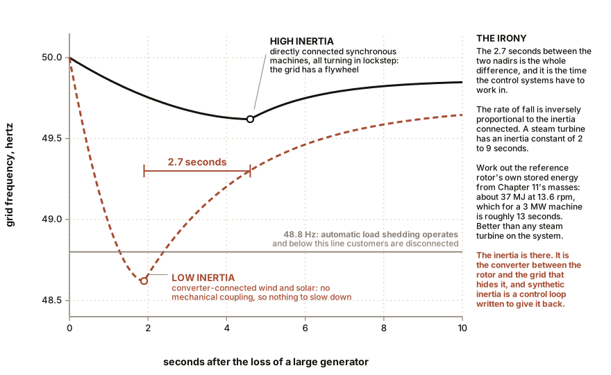
Which means the grid has a flywheel. If demand suddenly exceeds generation, the extra energy comes out of that stored rotation and everything slows down slightly. The frequency falls, and it falls at a rate set by how much rotating inertia is connected. That gives the control systems a few seconds to respond, and those few seconds are the entire reason the lights stay on.
The measure is the inertia constant H, the stored kinetic energy divided by the machine’s rating, in seconds. A steam turbine generator is typically 2 to 9 seconds. And the rate of change of frequency after a sudden loss of generation is inversely proportional to the total inertia connected, so a grid with less inertia falls faster and has less time to react.
Now the part that is a genuine irony. Work out our rotor’s stored kinetic energy from Chapter 11’s masses. Three blades of about 12 tonnes (13 tons) each, treated as rods pivoting at the hub, give a moment of inertia near 36 million kg per square metre, and at 13.6 rpm that is about 37 MJ, which for a 3 MW machine is an inertia constant in the region of 13 seconds, better than any steam turbine on the system.
And the grid cannot have any of it, because Chapter 12’s converter deliberately stands between the rotor and the grid so the rotor can chase its optimal tip-speed ratio. The flywheel is there, it is excellent, and it is electrically invisible.
The answers, and all three are real engineering in current deployment:
Synthetic inertia, sometimes called fast frequency response. The converter is programmed to detect a falling frequency and briefly inject extra power, taken from the rotor’s kinetic energy, slowing the rotor deliberately. It is not true inertia because it is a control loop with a detection delay rather than a physical coupling, but it can respond in well under a second, and some grid operators, notably in Quebec, have required it for years.
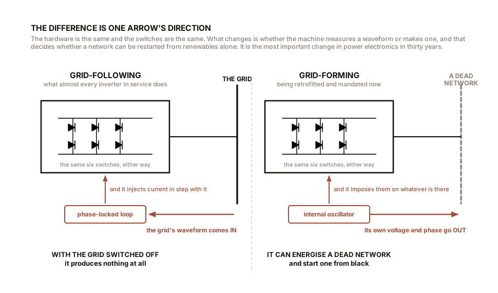
Grid-forming inverters. A conventional wind or solar inverter is grid-following: it measures the grid’s voltage waveform and injects current in step with it, so it needs the grid to already exist. A grid-forming inverter instead imposes its own voltage waveform, behaving like a synchronous machine, and can therefore hold up a network by itself and even start one from black. This is the most important change in power electronics in thirty years and it is being retrofitted and mandated now.
Synchronous condensers. The blunt answer: a large synchronous machine spinning with no prime mover attached, connected to the grid purely to supply inertia and short-circuit strength. Several have been built by converting the generators of retired coal plants, which is the grid buying back for money something it used to get for nothing.
Section 5: Two Blackouts, Read Properly
Two events are worth studying because both are usually described wrongly, and in both cases the honest reading is more useful than the political one.
South Australia, 28 September 2016. An extreme storm brought down twenty-three transmission towers. The network then experienced a rapid series of voltage dips as faults occurred. Nine wind farms then reduced their output almost simultaneously, shedding around 450 MW in seconds, because their protection settings limited how many voltage dips they would ride through before curtailing, and that limit had been reached. The sudden loss overloaded the interconnector to the neighbouring state, which tripped, and the whole state went dark. About 850,000 customers lost supply.
The honest reading is not that wind caused it. The storm caused it, and towers falling over is a fault condition any grid must survive. What the wind farms contributed was a protection setting that nobody had reviewed, a limit on ride-through events that was appropriate for a small number of machines on a strong grid and dangerous for a large number on a weak one. The settings were subsequently changed and the same event today would not produce the same outcome. Which is the point: it was a configuration failure in a system whose composition had changed faster than its settings.
Great Britain, 9 August 2019. Lightning struck a 400 kV circuit. The circuit cleared correctly in under a tenth of a second. In the seconds that followed, the Hornsea One offshore wind farm reduced output by several hundred megawatts and the Little Barford gas plant lost a steam turbine, and a large amount of small embedded generation disconnected on rate-of-change-of-frequency protection. Frequency fell to 48.8 Hz, below the threshold at which automatic low-frequency demand disconnection operates, and about a gigawatt of load was shed. Roughly 1.1 million customers were affected, including a substantial part of the rail network.
The honest reading here is about inertia and about protection coordination, not about wind being unreliable. The lightning strike was ordinary. What was not ordinary was how fast the frequency fell, which is Section 4’s inverse relationship with connected inertia, and how many small generators disconnected on protection settings that were themselves reacting to the falling frequency, making it fall further. A cascade of correct local decisions producing a wrong global outcome is the classic failure mode of a complex system, and it is a design problem rather than a technology verdict.
And the constructive part. South Australia’s response was, among other things, to install a large battery, initially 100 MW and 129 MWh, which turned out to be extraordinarily good at exactly the job Section 4 describes: responding in milliseconds to a frequency deviation. It substantially changed the economics of frequency regulation in that market. A battery does not solve the four-day Dunkelflaute of Section 3, and it solves the four-second problem beautifully, and keeping those two timescales distinct is most of the sense in this whole debate.
ON THE BENCH: Make a grid, and lose it
Section 4 is about inertia and synchronism, and both are demonstrable with two small motors and a piece of wire. This is one of the most instructive half hours in the book.
Parts: two identical small DC or brushless hobby motors used as generators, or better, two small three-phase brushless motors from a drone or a scrap printer; a large flywheel for one of them, which can be a heavy disc of MDF or a stack of washers, and nothing for the other; a low-voltage bulb or a resistor as the load; a variable bench supply or a battery and a potentiometer to drive them; a multimeter; a switch. Cost: $15 to $30. Time: 45 minutes. Hazards: low voltage only. Balance any flywheel before spinning it, and do not exceed the motor’s rated speed with mass on the shaft.
Method: 1. Spin one generator up to a steady speed with its flywheel fitted, and connect the load through the switch. Measure the voltage. 2. Now close the switch suddenly and watch both the voltage and the speed. Record how far the voltage dips and how long it takes to recover. 3. Remove the flywheel and repeat exactly the same step change.
What you should see: with the flywheel, the voltage dips a little and recovers. Without the flywheel, the same load step produces a much deeper and faster dip, because there is far less stored energy to bridge the gap while the drive catches up.
That is grid inertia, and you have just measured the difference between having it and not. The dip depth is the frequency excursion and the rate of the dip is the rate of change of frequency, and everything Section 4 says about a low-inertia grid is visible in the second trace.
If it does not work: if both cases look identical, your drive is too stiff and is holding the speed regardless. Drive the generator through a slipping rubber band or a weak spring coupling so the speed is genuinely free to sag.
Better, if you have one: two generators, both spinning, both feeding the same load through diodes, gives you a two-machine grid. Load it and see both slow together. Then disconnect one abruptly and watch the other take the whole load and sag much further. That is the 9 August 2019 event, in miniature, on a bench, for twenty dollars.
Section 6: Offshore, Which Is a Different Problem Rather Than the Same One Wet
It is tempting to describe offshore wind as onshore wind in water. Almost nothing carries across, and the differences are worth having in a list.
The wind is better and steadier. Chapter 9’s shear exponent offshore is about 0.10 against 0.20 or more on land, and turbulence intensity is 6 to 8 percent against 15 to 20. Both of those change the machine. Low shear means there is little to gain from a tall tower, so offshore hub heights are set by wave clearance and blade radius rather than by shear. Low turbulence means the fatigue budget of Chapter 9 is far less consumed by the wind, which is one of two reasons offshore blades can be so much longer.
The transport constraint disappears, which is the other reason. Chapter 11’s answer to why offshore blades are twice the length of onshore ones is not aerodynamics, it is that a ship does not turn corners. The largest offshore machines now use rotors over 230 m (755 ft) in diameter, sweeping over 40,000 square metres (430,000 square feet), rated at 14 to 15 MW. Compare that with this book’s 110 m (361 ft) onshore machine and note that the ratio in swept area is over four to one.
The foundation genuinely does rival the machine in cost, which Chapter 12 said was not true onshore. Three families, by water depth:
| Foundation | Water depth | What it is |
|---|---|---|
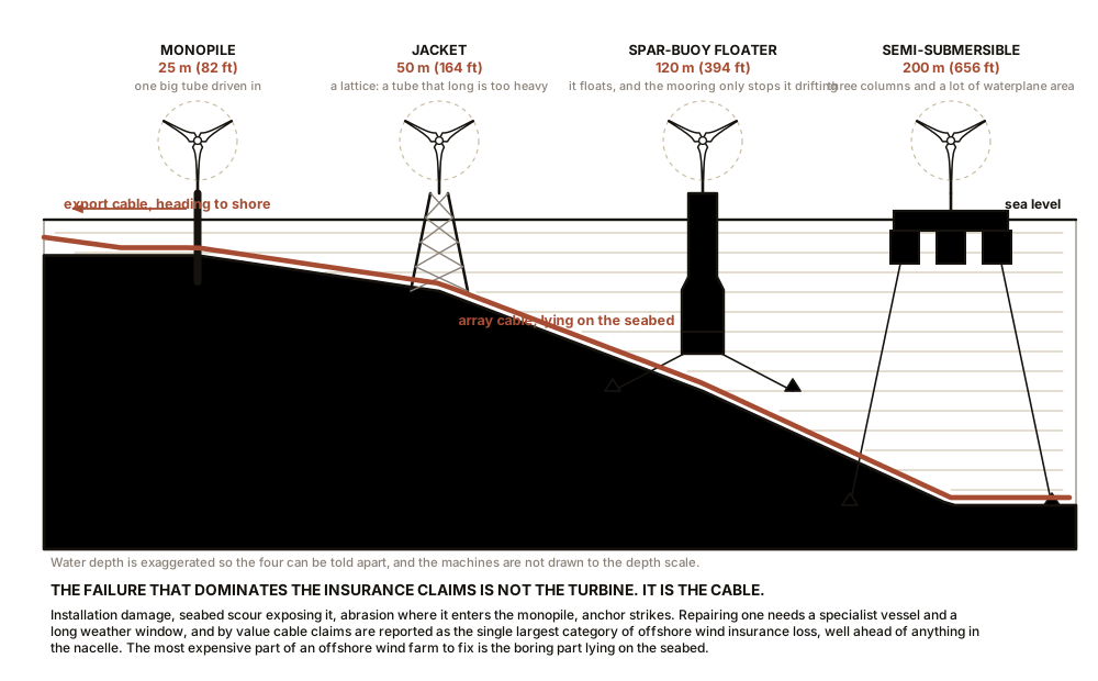
| Monopile | up to about 35 m (115 ft) | one large steel tube driven into the seabed, with a transition piece on top |
| Jacket | to about 60 m (200 ft) | a welded steel lattice on multiple piles |
| Floating | beyond that | a buoyant hull on catenary or taut moorings, with a dynamic export cable |
Floating is the frontier and it is genuinely new engineering, because a floating turbine’s controller must now handle a platform that pitches and heaves, and Chapter 13’s Region 3 pitch loop can, if badly tuned, actively pump energy into the platform’s motion and make it worse. Hywind Scotland, commissioned in 2017 with five machines on spar buoys, was the first commercial floating array.
Everything about access is different. A crew transfer vessel can typically only put technicians onto a turbine in significant wave heights up to around 1.5 m (5 ft), which in a North Sea winter can rule out access for weeks. That single constraint drives an enormous amount of design: it is why offshore machines favour direct drive to eliminate the gearbox, why condition monitoring is far more elaborate, why service operation vessels with motion-compensated gangways exist, and why offshore availability figures are lower than onshore despite better hardware.
And the failure that dominates the insurance claims is not the turbine. It is the cable. Subsea export and array cables suffer from installation damage, seabed scour exposing them, abrasion at the entry to the monopile, and anchor strikes, and repairing one requires a specialist vessel and a long weather window. By value, cable claims have been reported as the single largest category of offshore wind insurance loss, well ahead of any component in the nacelle. The most expensive part of an offshore wind farm to fix is the boring part lying on the seabed, which is a sentence worth remembering whenever a technology is judged by its most photogenic component.
SLOW DOWN. Check Your Understanding: A country reports that wind supplied 55 percent of its electricity last year. A critic responds that since wind’s capacity factor is only about 40 percent, the country must be relying on imports for the other 45 percent and the figure is misleading. Is the critic right? Think it through before reading on.
No, and the error is a confusion between two completely different fractions that happen to be percentages.
Capacity factor is a fraction of a machine’s own nameplate over time. Generation share is a fraction of a country’s electricity. They are not comparable and neither constrains the other, because the missing variable is how much capacity was installed.
Work it out. If a country’s demand averages 4 GW, and it installs 5.5 GW of wind capacity at a 40 percent capacity factor, that wind fleet produces an average of 2.2 GW, which is 55 percent of 4 GW. There is no contradiction and no import required on an annual basis. A capacity factor of 40 percent simply means you install roughly two and a half times as much nameplate as the average output you want, which is exactly what the countries with high wind shares have done.
What the critic is groping toward is a real problem, and it is not this one. The real problem is Section 3’s fourth item: the annual average balances and the individual hour does not. In a windy hour that fleet produces well over demand and must curtail or export; in a calm week it produces almost nothing and something else must run. The challenge of a high-wind system is entirely about matching within hours and days, and not at all about matching over a year.
Which is why the annual generation share, the very number the argument started with, is nearly useless as a measure of how hard the problem is. The numbers that matter are the size of the largest sustained low-wind event, the correlation between wind and demand, and the amount of firm capacity or storage held for the handful of days when the first two are unkind. A country at 55 percent annual wind share with strong interconnection and hydro storage has an easier system than a country at 30 percent with neither, and no capacity factor anywhere reveals that.
Chapter 17 stops asking how the machine works and asks how it stops working, which is the question that decides whether any of the economics in this chapter was real.

Bench Degree
Get the degree without the diploma.
Learn the material, not how to pass the exam.