Bench Degree·WIND POWERchapter

Chapter 10: The Distribution
The average wind speed at a site is close to useless on its own. This chapter shows you why, and gives you the two numbers that are not useless, and both of them you can measure yourself with a logger and a week.
Chapter 9 gave you the wind as a shape: faster with height, rougher near obstacles, slower behind a neighbour. This chapter gives you the wind as a spread of speeds, which is the form in which it actually pays.
The reason the distinction matters is Chapter 1’s cube law. A quantity that rises as the cube of speed cannot be computed from an average speed, and the error is not a few percent. At an ordinary temperate site it is nearly a factor of two, and it runs in the direction that flatters whoever is selling the project.
Section 1: The Distribution, Which Is the Point of the Chapter
Here is the fact that governs everything, and it is worth a section on its own.
An average wind speed, on its own, is nearly meaningless.
Consider two sites, both with an annual mean wind speed of 7 m/s (16 mph). Site A is a steady trade-wind coast where the wind is between 6 and 8 m/s (13 and 18 mph) almost all year. Site B is a continental plain that is calm half the time and blowing 14 m/s (31 mph) the other half.
They have the same mean. Site B has nearly twice the energy, because power goes as the cube and the cube of the average is not the average of the cube.
Arithmetic, at its crudest: for Site A take a constant 7 m/s (16 mph), so the mean cube is 343. For Site B, half the time zero and half the time 14 m/s (31 mph), so the mean cube is half of 2,744, which is 1,372. Four times the energy for the same mean. That is an extreme example and the direction of the effect is general.
So the wind resource at a site is a distribution and not a number, and the distribution that the industry uses to describe it is the Weibull distribution:
f(v) = (k/c) (v/c)^(k−1) exp( −(v/c)^k )Two parameters. c is the scale parameter, in units of speed, and it sits a little above the mean. k is the shape parameter, dimensionless, and it says how spread out the wind is. Low k means broadly spread with lots of calms and lots of gales. High k means concentrated near the mean.
| k | Character | Where |
|---|---|---|
| 1.2 to 1.5 | Very broad; long calms and strong storms | monsoon and continental interiors |
| 2.0 | The standard temperate case, also called Rayleigh | most of northern Europe and North America |
| 2.5 to 3.0 | Narrow, steady | trade wind coasts and islands |
| 3.5+ | Very steady | some Caribbean and Pacific sites |
And now the number that makes the whole thing concrete. For a Weibull distribution, the ratio of the mean of the cube to the cube of the mean, which is called the energy pattern factor, comes out as a pure function of k:
| k | mean of v³, divided by the cube of the mean v |
|---|---|
| 1.5 | 2.72 |
| 2.0 | 1.91 |
| 2.5 | 1.58 |
| 3.0 | 1.40 |
| 4.0 | 1.24 |
Read the k = 2 row. At an ordinary temperate site, the wind carries 1.91 times the energy that its average speed alone would suggest. Not five percent more. Ninety-one percent more, almost double.
Worked, for the site this book will use throughout. Mean wind speed 7 m/s (16 mph), k = 2. The scale parameter c works out at 7.9 m/s (17.7 mph).
- Power computed from the mean speed: 0.6125 × 343, which is 210 W per square metre (19.5 W per square foot).
- Power computed from the distribution: 0.6125 × 655, which is 401 W per square metre (37.3 W per square foot).
Two hundred and ten against four hundred and one. An engineer who sized a project on the first number would have got it wrong by nearly a factor of two, in the direction that loses money for the person who told them it was fine.
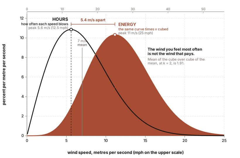
One caution so the book stays honest. A real turbine cannot take all of that, because Chapter 13’s power curve goes flat above rated speed and deliberately declines the strongest winds. So the distribution roughly doubles the energy in the wind, and the machine’s rated ceiling gives some of it back, and the only number that captures both is Chapter 16’s capacity factor. Never quote a resource figure as though it were a yield figure. That single confusion is responsible for more failed small-wind projects than any hardware defect.
ON THE BENCH: Log a week and draw your own distribution
This is the most valuable measurement in the book and the least dramatic. It takes seven days of doing nothing and it will change how you read every wind claim you ever see again.
Parts: a logging anemometer, or a cheap cup anemometer with a pulse output wired to a microcontroller board, or a hand anemometer and a stubborn habit; a mast or pole to get the sensor at least 2 m (6.5 ft) above the ground and well clear of the house; a spreadsheet. Cost: $30 for a hand anemometer and a notebook, $60 to $150 for a logging unit with a data output, and the logging unit is worth it. Time: an hour to install, seven days of waiting, an hour to plot. Hazards: anything on a mast can blow down. Guy it. Do not put anything on a roof in a wind you would not stand in.
Method: 1. Mount the anemometer clear of obstructions, ideally at ten times the height of anything within a few metres of it, which you will not manage, so record what is nearby and accept that you are measuring your garden and not your region. 2. Log wind speed every ten minutes for seven days. If you are doing it by hand, six readings a day at set times, for a month, gets you something usable. 3. Put the readings in bins 1 m/s (2.2 mph) wide and plot the histogram. 4. Compute two numbers. First, the mean of all your readings, cubed. Second, the mean of the cubes of all your readings. These are one spreadsheet column each.
What you should see: a histogram that rises from zero, peaks somewhere below the mean, and trails off to the right with a long thin tail. That is a Weibull distribution and you did not have to assume it. And the mean of the cubes will be between one and a half and three times the cube of the mean. Divide one by the other and you have measured your own site’s energy pattern factor.
The lesson, which is worth the week: the handful of windiest hours in your log will hold a startling share of the total energy. Sort your readings by speed, take the top ten percent, and add up their cubes. At an ordinary site the windiest ten percent of the time carries something like a third to a half of all the energy. That is why a turbine’s behaviour in strong wind matters so much more than its behaviour in a breeze, and it is Chapter 13’s entire subject.
Better, if you have one: log at two heights on the same mast, say 2 m and 4 m (6.5 ft and 13 ft). Take the ratio of the means, and solve for α. You have measured your own shear exponent, and you can now estimate what a tower would buy you.
Section 2: The Wind at Night, Which Nobody Expects
One more fact, because it surprises everybody and it has real consequences.
Chapter 9 Section 1’s shear exponent is not a constant for a site. It changes through the day, and dramatically.
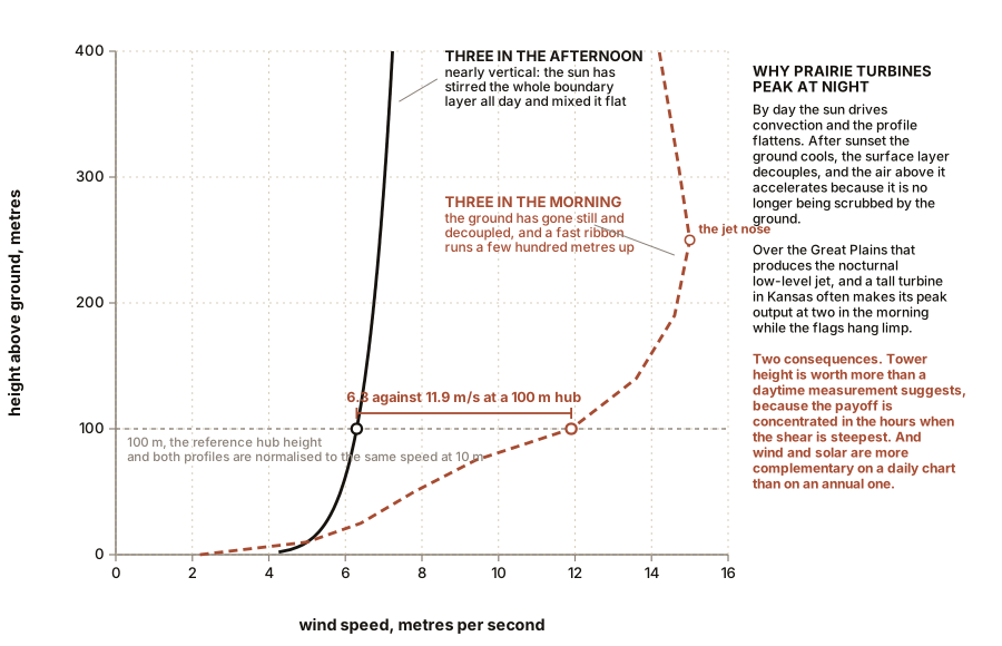
In daytime the sun heats the ground, the ground heats the air, the warm air rises and the boundary layer mixes vigorously. Mixing carries fast air down and slow air up, so the profile flattens and shear is low. By late afternoon α at a farmland site may be 0.1 or less.
At night the ground cools by radiation, the air near it cools, and a stable layer forms that resists vertical mixing. The air above is now decoupled from the ground’s friction and accelerates, sometimes to well above the geostrophic speed, while the air near the ground goes still. Shear becomes extreme, with α reaching 0.4 or higher.
Over the Great Plains of the United States this produces the nocturnal low-level jet, a ribbon of fast air a few hundred metres up that peaks in the small hours. The consequence is that a tall turbine in Kansas or Oklahoma often produces its peak output at two in the morning, while at ground level the flags hang limp.
Two consequences worth carrying. First, the value of tower height is much greater than a daytime measurement suggests, because the payoff is concentrated in the hours when the shear is steepest. Second, wind and solar are less complementary than they look on an annual chart and more complementary than they look on a daily one, because a continental wind resource often peaks precisely when the panels are dark. Chapter 16 uses that.
SLOW DOWN. Check Your Understanding: A developer measures a site for one year with a 60 m (197 ft) met mast and reports a mean wind speed of 7.0 m/s (15.7 mph). A second developer measures the same site the following year and reports 6.4 m/s (14.3 mph). Neither made a mistake. Which of them should the bank believe, and what should the bank actually ask for? Answer before reading on.
Neither, and the bank should ask for a long-term correlation.
Year-to-year variation in mean wind speed at a fixed site is real and substantial: a standard deviation of 5 to 6 percent between consecutive years is normal, and a decade can easily contain a year 15 percent above and a year 15 percent below the long-run mean. Both developers measured honestly. They measured different years.
And the cube law turns a modest measurement question into a project-killing one. A drop from 7.0 to 6.4 m/s (15.7 to 14.3 mph) is 8.6 percent in speed, and by Chapter 17’s arithmetic that costs roughly 15 percent of annual energy once the power curve is applied. A project financed at the higher figure and delivering the lower one has lost most of its margin.
So what the industry actually does, and what the reader should ask for by name, is measure-correlate-predict. You take a year of on-site data, correlate it against twenty or thirty years of data from a nearby long-term reference such as an airport or a reanalysis dataset, and use the correlation to estimate what the site’s long-run mean would have been. The output is not a mean, it is a mean with a stated uncertainty and a stated exceedance probability, and the honest form is “P50 of 6.7 m/s (15.0 mph), P90 of 6.2 m/s (13.9 mph)”, meaning there is a fifty percent chance of beating the first and a ninety percent chance of beating the second.
The general point is bigger than wind. One year of good data about a variable process is not a measurement of the process, it is one sample from it. Anybody who quotes you a single-year average without an uncertainty has not finished the measurement, and Chapter 17 shows what happens to projects built on unfinished measurements.
Chapters 11 and 12 stop looking at the air and open the machine, part by part, from the blade root bolts to the concrete in the ground.

Bench Degree
Get the degree without the diploma.
Learn the material, not how to pass the exam.