Bench Degree·WIND POWERchapter

Chapter 13: The Power Curve
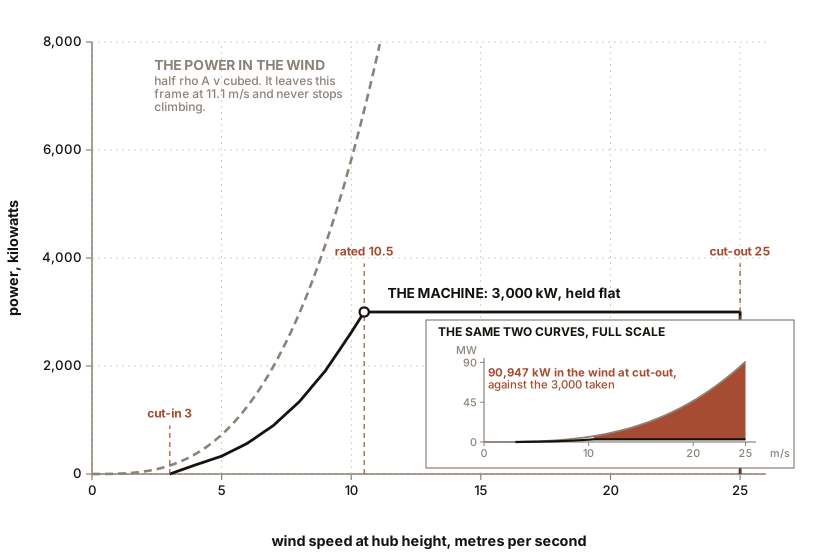
In a 56 mph gale there is 91 MW of wind going through this machine’s rotor and it is taking three. That is not a limitation, it is the most deliberate decision in the whole design, and this chapter is why.
Everything in this book so far has been about how much a turbine can take. This chapter is about the far more interesting question of how much it chooses to take, and when it refuses.
The answer lives in one diagram, the power curve, and a reader who can read one properly can interrogate any turbine specification in the world.
Section 1: The Power Curve, Read Properly
A power curve plots electrical output against wind speed at hub height. Here is the one for the machine this book has been building: 3 MW, 110 m (361 ft) rotor, 9,503 square metres (102,290 square feet) swept, overall power coefficient 0.45 at its best point.
| Wind speed | Power in the wind | Machine output | |
|---|---|---|---|
| 3 m/s | 7 mph | 157 kW | 0 (cut-in) |
| 4 m/s | 9 mph | 373 kW | 170 kW |
| 5 m/s | 11 mph | 728 kW | 330 kW |
| 6 m/s | 13 mph | 1,258 kW | 570 kW |
| 7 m/s | 16 mph | 1,997 kW | 900 kW |
| 8 m/s | 18 mph | 2,981 kW | 1,340 kW |
| 9 m/s | 20 mph | 4,244 kW | 1,910 kW |
| 10 m/s | 22 mph | 5,821 kW | 2,620 kW |
| 10.5 m/s | 23 mph | 6,738 kW | 3,000 kW (rated) |
| 15 m/s | 34 mph | 19,645 kW | 3,000 kW |
| 20 m/s | 45 mph | 46,565 kW | 3,000 kW |
| 25 m/s | 56 mph | 90,947 kW | 0 (cut-out) |
One detail in that table repays a look. The overall power coefficient peaks at 0.45 a little below rated and has slipped to 0.445 by the time rated power is reached, which is Region 2.5 of the next section giving up a sliver of capture to stay under the tip-speed limit. A real power curve is never a clean multiple of the wind’s cube, and the places where it departs are all decisions.
Three speeds have names and all three are design choices rather than natural facts.
Cut-in speed, 3 m/s (7 mph) here. Below this the machine does not generate. The reason is not that it cannot turn, it is that it cannot turn profitably. At 3 m/s (7 mph) there is 157 kW in the wind and 0.45 of that is 71 kW, from which you must subtract drivetrain losses at partial load, and then subtract the machine’s own parasitic consumption: yaw drives, pitch drives, controller, cooling pumps, oil heaters, the dehumidifier in the nacelle, aviation lights. That can be 10 to 30 kW. Below cut-in the machine would be a net consumer, so it idles.
Rated speed, 10.5 m/s (23 mph) here. The lowest wind speed at which the machine produces its nameplate power. Above this the output is deliberately held flat.
Cut-out speed, 25 m/s (56 mph). The machine shuts down entirely, feathers its blades and parks. Chapter 14 Section 2 is entirely about why.
Section 2: The Four Regions, and the Cleverest Trick in the Machine
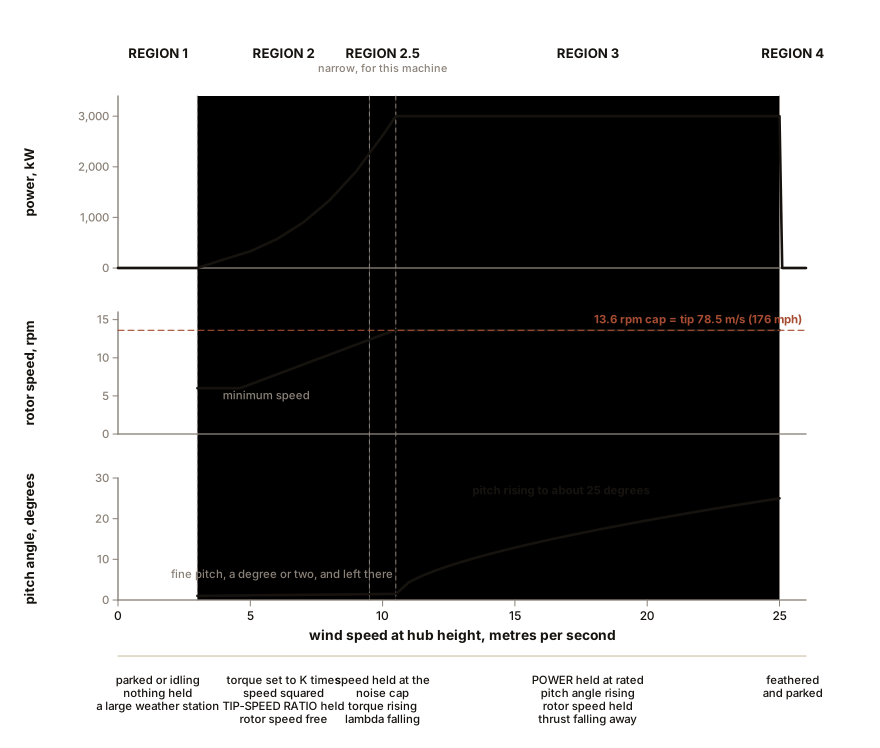
A modern variable-speed pitch-controlled turbine operates in four distinct regions, and the controller behaves like a different machine in each.
Region 1, below cut-in. The rotor idles or is parked. Blades are pitched to a low-torque position, the generator is offline, and the machine is a large weather station.
Region 2, cut-in to about 9 m/s (20 mph): variable speed at constant tip-speed ratio. This is where the beautiful part lives.
Chapter 6 established that a fast rotor has a sharp peak in its power coefficient against tip-speed ratio curve, so to stay at that peak the rotor speed must be proportional to the wind speed. Which raises an obvious problem: the anemometer on the nacelle roof is one point measurement in a turbulent flow behind a rotor, and it is nowhere near good enough to command rotor speed from.
So the controller does not use it. Here is the trick.
Chapter 1’s equation, with a power coefficient, is
P = ½ρπR²v³C_P. If the rotor is sitting at its optimal
tip-speed ratio then v = ωR/λ_opt. Substitute:
P = ½ ρ π R⁵ (C_P,max / λ_opt³) ω³and torque is power divided by rotational speed, so
T = K ω² with K = ½ ρ π R⁵ C_P,max / λ_opt³Read what that says. If the controller simply commands the generator to apply a torque proportional to the square of the measured rotor speed, with the constant K computed once from the rotor’s geometry, then the rotor finds and holds its own optimal tip-speed ratio in any wind, with no wind measurement whatever.
The feedback is physical rather than computational. If the wind
rises, the aerodynamic torque exceeds Kω², the rotor
accelerates, Kω² rises to meet it, and the rotor settles at
a higher speed with λ unchanged. If the wind drops, the reverse.
The rotor speed is the wind measurement, and it is a
far better one than any anemometer, because it is an average over the
whole 9,503 square metre (102,290 square foot) disc rather than a sample
at one point.
For our machine, with R of 55 m (180 ft), a maximum aerodynamic power coefficient of 0.49 and an optimal λ of 7.5, K comes out at about 1.13 million in units of newton metres per radian per second squared. At rated, ω is 1.43 radians per second, so T is 1.13 million times 2.04, which is 2.3 MN·m, matching Chapter 11’s figure exactly, which is how you know the arithmetic closed.
IN PLAIN ENGLISH: The turbine keeps its blades at exactly the right speed for the wind, and it does it without knowing how hard the wind is blowing. It just pulls back on the generator harder when the rotor speeds up, in a fixed ratio, and the physics does the rest. It is the same trick as a bicycle finding its own speed when you hold a steady effort on the pedals.
Region 2.5, about 9 to 10.5 m/s (20 to 23 mph): constant speed, rising torque. The rotor has reached the maximum speed it is allowed, set by the tip-speed limit of Chapter 6, which onshore is a noise limit. It can go no faster, so the controller holds the speed and lets the torque rise. Tip-speed ratio now falls below optimal and a little power coefficient is sacrificed, deliberately, to stay under the noise limit.
Region 3, above rated: constant power. The controller pitches the blades to shed exactly as much lift as necessary to hold the output at 3 MW, and no more. As the wind rises the pitch angle increases, from a fine angle of a few degrees at rated to perhaps 25 degrees at cut-out. Output stays flat while the wind’s power climbs by a factor of thirteen.
Region 4, above cut-out. Shut down and parked. Or, on newer machines, Chapter 14’s storm control.
Section 3: Why Flat, Which Is the Chapter’s Real Question
Look at the last three rows of Section 1’s table again. At 25 m/s (56 mph) there is 91 MW in the wind through that rotor and the machine takes 3 MW. Even at 0.45 it could in principle take 41 MW.
Why on earth would you leave 38 MW on the table?
Because you would have to buy a drivetrain fourteen times bigger to catch it, and it would be idle almost all the time.
Everything downstream of the blades is sized by power, not by wind: the gearbox, the generator, the converter, the transformer, the tower cable, the grid connection. A 41 MW drivetrain in this rotor would cost several times the whole machine.
And how much energy would it earn? Chapter 10’s distribution answers that. At our reference site, mean 7 m/s (16 mph) with a Weibull shape factor of 2, the wind blows above 25 m/s (56 mph) for a matter of hours a year, and those hours carry well under one percent of the site’s annual energy.
Fourteen times the drivetrain, for under one percent more energy. Stated that way it is not a difficult decision, and it is the same decision every generating technology makes: you size the machine for a duty cycle, not for the extreme.
There is a more elegant way to say the same thing. Rated power is not a limit the designer accepted, it is a variable the designer chose, and choosing it is the single most consequential economic decision in a turbine’s design. Choose it high and you get a machine that rarely reaches nameplate, sold as a big number, with a low capacity factor. Choose it low and you get a machine that sits at nameplate for a fifth of the year, with a high capacity factor and a smaller number on the label.
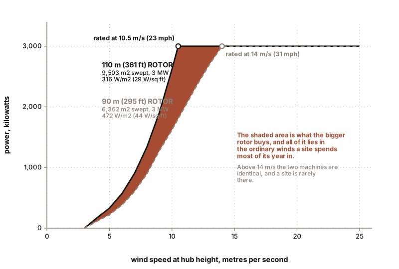
The industry has moved decisively toward the second, and the measure of it is specific power, the rated power divided by the swept area:
| Era and type | Specific power |
|---|---|
| 1990s onshore | 450 to 550 W per square metre (42 to 51 W per square foot) |
| 2010s onshore | 350 to 400 W per square metre (33 to 37 W per square foot) |
| Our machine, modern onshore | 316 W per square metre (29 W per square foot) |
| Modern high-capacity-factor onshore | 200 to 280 W per square metre (19 to 26 W per square foot) |
A lower number means a bigger rotor on a smaller generator, which means the machine reaches rated in a gentler wind and holds it for far more of the year. It produces less at its very best moment and much more over a year. Chapter 16 shows that this single trend, and not any improvement in aerodynamics, is where most of the last twenty years of capacity factor gains came from.
ON THE BENCH: Plot your own power curve
Every element of Section 1 is measurable on a card rotor. What you will get is the right shape with the wrong numbers, and Chapter 4 Section 6 already told you why.
Parts: your three-blade winged rotor and motor; a box fan with three or more speeds, or better, a fan on a mains dimmer or a variable-speed bench fan; a vane anemometer; a decade resistance box, or a set of resistors from 10 to 1,000 ohms, or a wirewound potentiometer of about 500 ohms rated a few watts; a multimeter, ideally two. Cost: $25 for a resistor set and an anemometer if you lack them. Time: two hours to take a full curve, and take it twice. Hazards: the fan intake. A dimmer on an induction motor can overheat it; use a fan rated for speed control, or just use its own speed switch and accept three points.
Method: 1. Set the fan to its lowest speed. Measure the air speed at the rotor plane with the rotor removed. 2. Fit the rotor. Sweep the load resistance across its whole range, and at each value record voltage across the resistor. Power is voltage squared divided by resistance. Find the resistance that gives maximum power and note it. 3. That maximum is the machine’s output at that wind speed. Record the pair. 4. Repeat for every fan speed you can produce. 5. Plot power against air speed on paper.
What you should see: a curve that rises steeply and is well fitted by a cube law over the range you can reach. Try it: divide each power by the cube of its air speed and the answers should be roughly constant. You have measured the exponent in Chapter 1’s equation for the third time and this time you have measured it as a curve rather than as two points.
What you will not see is a flat top, because your rotor has no rated power, no pitch system and no controller. Which is itself the lesson. An uncontrolled rotor’s output follows the wind’s cube for as long as the wind rises and the machine survives, and every flat power curve in the world is flat because somebody decided it should be.
If it does not work: if power does not peak with load resistance but rises monotonically, your load range is too narrow. Add a lower-value resistor. If the rotor stalls and stops when loaded, you are past the peak of the tip-speed ratio curve, which is Chapter 6’s sharp peak and is worth noting as a finding rather than a failure.
Better, if you have one: a second multimeter measuring current lets you take real power directly instead of inferring it, and a photo tachometer lets you plot tip-speed ratio against load. Then you can put the optimal-torque law of Section 2 to the test: check whether the torque at the best point really does go as the square of the rotational speed across your fan speeds. That is a genuinely satisfying afternoon.
SLOW DOWN. Check Your Understanding: Two turbines stand side by side at the same site. Both have a 110 m (361 ft) rotor. One is rated at 3 MW and one at 4.5 MW, and the 4.5 MW machine costs 12 percent more. Which produces more electricity in a year, and which reports the better capacity factor? Answer both before reading on, and then decide which you would buy.
The 4.5 MW machine produces about 17 percent more energy in a year. It reports a capacity factor of about 30 percent against the 3 MW machine’s 39 percent.
Work through why. Both machines have the same rotor, so below 10.5 m/s (23 mph) their power curves are identical, point for point. The 4.5 MW machine simply keeps climbing past that point up to a rated speed near 12 m/s (27 mph), and above that it holds 4.5 MW instead of 3 MW. Everything it gains, it gains in winds above 10.5 m/s (23 mph), and Chapter 10’s distribution says those winds are 20 percent of the hours and rather more of the energy. Integrating our reference site’s Weibull distribution against both curves gives 1,169 kW average for the 3 MW machine and 1,364 kW for the 4.5 MW machine.
Now the two conclusions, and they point in opposite directions.
On cost per kilowatt-hour, the 4.5 MW machine wins at this price. Seventeen percent more energy for twelve percent more money is a better deal. If the premium were twenty percent instead, which is closer to what a fifty percent larger drivetrain, transformer and grid connection usually cost, the answer would reverse. The verdict turns entirely on a number the question handed you, and that is the point: this is an arithmetic question and not a matter of principle.
And on capacity factor, the 4.5 MW machine loses badly while producing more electricity. Its energy went up by 17 percent and its nameplate went up by 50 percent, so the ratio between them fell. The machine with the far worse capacity factor is the one making more power.
Which is why Chapter 16 spends a section insisting that capacity factor is not an efficiency and not a quality score. It is a ratio whose denominator is a marketing decision.
One further subtlety, because it is the thing people get backwards. Section 3 said the industry has moved toward low specific power, meaning big rotors on modest generators, and that sounds like the opposite of what this question just concluded. It is not, because the two comparisons hold different things fixed. This question fixed the rotor and varied the nameplate. Section 3 fixed the nameplate and varied the rotor. Swept area is cheap per unit and drivetrain is expensive per unit, so the winning move is always toward more rotor and less generator, and both comparisons say exactly that when you read them the same way round.
So the flat top of a power curve is a decision about money, and the four regions are how a controller carries that decision out. What none of it says is how the blades are actually made to shed the lift, and there are two entirely different philosophies about that, one of which has almost won. Chapter 14 sets them against each other, and then follows the machine into the storm.

Bench Degree
Get the degree without the diploma.
Learn the material, not how to pass the exam.